Applications of an exact counting formula in the Bousso-Polchinski Landscape

Abstract

The Bousso-Polchinski (BP) Landscape is a proposal for solving the Cosmological Constant Problem. The solution requires counting the states in a very thin shell in flux space. We find an exact formula for this counting problem which has two simple asymptotic regimes, one of them being the method of counting low $\Lambda$ states given originally by Bousso and Polchinski. We finally give some applications of the extended formula: a robust property of the Landscape which can be identified with an effective occupation number, an estimator for the minimum cosmological constant and a possible influence on the KKLT stabilization mechanism.

1 Introduction

The eternal inflation picture of the multiverse consists of de Sitter bubbles nucleating in certain vacuum state of very high energy density [1, 2, 3, 4, 5]. Bubbles can be created inside other bubbles, and this provides a dynamical relaxation mechanism which gives rise to an average neutralization of the cosmological constant [6, 7]. We may wonder if it’s possible to formulate a model of eternal inflation with relaxation containing vacuum states of a cosmological constant as small as the observed value [8, 9]

$$\Lambda_{\text{obs}}=1.5\times 10^{-123}\,,$$ (1)

without fine-tuning the parameters of the model and avoiding the need of invoking the anthropic principle [10, 11, 12], which has been used to explain why we are living in such a special region of the multiverse. The smallness of the number in (1) is the cosmological constant problem [13, 14]. An attempt for a solution is given in the Bousso-Polchinski Landscape [15], in which a large amount $J$ of quantized fluxes of charges $\{q_{j}\}_{i=1,\cdots,J}$ leads to an effective cosmological constant

$$\Lambda=\Lambda_{0}+\frac{1}{2}\sum^{J}_{j=1}n_{j}^{2}q_{j}^{2}\,.$$ (2)

In (2), $\Lambda_{0}$ is a negative number of order $-1$, and the integer $J$-tuple $(n_{1},\cdots,n_{J})$ characterizes each of the vacua of the Landscape. Without fine-tuning, for large $J$ and incommensurate charges $\{q_{j}\}$ this model contains states of small $\Lambda$. The problem arises now as how to count them. Unfortunately, the amount of these anthropic states is expected to be very small as compared to the total number of vacua in the Landscape [17], and therefore it seems not to be other way out but invoking the anthropic principle to explain the value (1).

The states in the Bousso-Polchinski Landscape can be viewed as nodes of a lattice in flux space $\mathbb{R}^{J}$. We call this lattice $\mathcal{L}$ and the charges $q_{i}$ are the periods of $\mathcal{L}$, that is,

$$\mathcal{L}=\bigl{\{}(n_{1}q_{1},\cdots,n_{J}q_{J})\in\mathbb{R}^{J}\colon n_{1},\cdots,n_{J}\in\mathbb{Z}\bigr{\}}\,.$$ (3)

A single state $\lambda$ in this lattice is characterized by the quantum numbers $(n_{1},\cdots,n_{J})$, and its cosmological constant is, according (2),

$$\Lambda(\lambda)=\Lambda_{0}+\frac{1}{2}\|\lambda\|^{2}\,.$$ (4)

Vacuum states in the Bousso-Polchinski Landscape are defined in the semiclassical approximation as stationary points of an effective action. If we consider two neighbor states of very high $\Lambda$ (neighbor states have quantum numbers $\{n_{j}\}$ which are different at one place and by one unit) we find that the energy barrier separating them is small, that is, the mediating Brown-Teitelboim instanton has a comparatively low action. These states are not isolated and consequently the semiclassical approximation breaks down for them. Moreover, when $\Lambda$ reaches a value near the Planck energy density (of order $\Lambda\approx 1$), quantum gravity effects become important, and some approximations made in the Bousso-Polchinski model (as neglecting the backreaction effect, for example) are no longer valid.

Thus the Bousso-Polchinski Landscape is a finite subset (yet an enormous one, a commonly quoted number being $10^{500}$ [18, 19, 20, 21]) of the lattice (3), comprising the nodes with cosmological constant smaller than some value $\Lambda_{1}=\mathcal{O}(1)$.

We will review the counting argument of Bousso and Polchinski [15, 16]. Around each node $\lambda$ of the lattice $\mathcal{L}$ we have a Voronoi cell which is a translate of the parallelotope $Q=\prod^{J}_{i=1}[-\frac{q_{i}}{2},\frac{q_{i}}{2}]$ of volume $\operatorname{vol}Q=\prod^{J}_{i=1}q_{i}$. On the other hand, each value of the cosmological constant $\Lambda_{0}\leq\Lambda\leq\Lambda_{1}$ defines a ball $\mathcal{B}^{J}(R_{\Lambda})$ in flux space of radius $R_{\Lambda}=\sqrt{2(\Lambda-\Lambda_{0})}$, and whose volume is

$$\operatorname{vol}\mathcal{B}^{J}(R_{\Lambda})=\frac{R_{\Lambda}^{J}}{J}\operatorname{vol}S^{J-1}\,,$$ (5)

where the volume of the $J-1$ sphere is

$$\operatorname{vol}S^{J-1}=\frac{2\pi^{\frac{J}{2}}}{\Gamma\bigl{(}\frac{J}{2}\bigr{)}}\,.$$ (6)

The BP counting argument consists of computing the number of states inside a ball of any radius $r$, which will be called $\Omega_{J}(r)$, by taking the quotient between the volume of the ball and the volume of the cell of a single state:

$$\Omega_{J}(r)=\frac{\operatorname{vol}\mathcal{B}^{J}(r)}{\operatorname{vol}Q}\,.$$ (7)

Plugging in some numbers, if $\Lambda_{0}=-1$, $\Lambda_{1}=1$, $J=300$ and $q_{i}=\frac{1}{10}$, we have a BP Landscape with

$$\Omega_{300}(2)=1.3\times 10^{202}\quad\text{states}\,.$$ (8)

This is certainly very small when compared with $10^{500}$. But if we take a charge ten times smaller $q_{i}=0.01$, we obtain $\Omega_{300}(2)=1.3\times 10^{502}$. Nevertheless, there is another argument which gives a more impressive number. The quotient between $2R_{\Lambda_{1}}$ and $q_{i}$ gives the number of nodes that fit in axis $i$. So, the total number of nodes is the product of all these quotients, which is also the volume of the hypercube of side $2R_{\Lambda_{1}}$ divided by the volume of the cell. With the same numbers this quantity is $4.1\times 10^{480}$. This argument is wrong though, because the vast majority of the nodes of the hypercube lie outside the sphere of radius $R_{\Lambda_{1}}$, and thus they are not states of the Landscape.

We may wonder how many states there are with values of $\Lambda$ comprised between 0 and a small positive value of the cosmological constant $\Lambda_{\varepsilon}$. Following the same argument as in the preceding paragraph, we compute the quotient between the volume of the shell comprised between radii $R_{0}=\sqrt{2|\Lambda_{0}|}$ and $R_{\varepsilon}=\sqrt{2(\Lambda_{\varepsilon}-\Lambda_{0})}\approx R_{0}+\frac{\Lambda_{\varepsilon}}{R_{0}}$ and we obtain

$$\mathcal{N}_{\varepsilon}=\Omega_{J}(R_{\varepsilon})-\Omega_{J}(R_{0})\approx R_{0}^{J-2}\,\frac{\operatorname{vol}S^{J-1}}{\operatorname{vol}Q}\,\Lambda_{\varepsilon}\,.$$ (9)

If $\Lambda_{\varepsilon}$ is of the order of the observed value (1), with the previous numbers we obtain $\mathcal{N}_{\varepsilon}=2.1\times 10^{36}$. Thus, if the degeneracy of these states is smaller than this number, we can find states with a realistic cosmological constant.

Nevertheless, as the authors of [15] point out, this argument is not valid when any of the charges $q_{i}$ exceed $R_{0}/\sqrt{J}$. We can see that strange things happen as $J$ grows with all the charges fixed. There is a critical value of $J$ above which the volume of the sphere is smaller than the volume of a single cell,

$$\operatorname{vol}\mathcal{B}^{J}(R_{0})<\operatorname{vol}Q\,,$$ (10)

and thus computing their quotient is not useful for counting. From inequality (10) we have

$$\frac{Jq^{2}}{R_{0}^{2}}>2\pi e>17$$ (11)

with $q=\sqrt[J]{\operatorname{vol}Q}$. Other strange thing happen for large $J$. Let’s assume for simplicity that all charges are equal to $q$. The corner of the cell centered at the origin is located at a distance $\frac{q}{2}\sqrt{J}$ from it, and it reaches (and surpasses) the radius $R_{0}$ when

$$\frac{Jq^{2}}{R_{0}^{2}}>4\,,$$ (12)

so we can expect the angular region near the corner to be devoid of states. Thus, the distribution of low $\Lambda$ states is not isotropic in flux space, and in particular, it has no spherical symmetry.

All these conditions coincide: when the parameter $h=\frac{Jq^{2}}{R^{2}}$ is large we cannot count by dividing volumes. But there are instances of the BP Landscape in which the parameter $h$ can be large and nevertheless the model contains a huge amount of states. In such cases the formula (7) should not be used, and another formula is needed. Other counting methods in the BP Landscape have been proposed so far [16, 17, 22, 23, 24], but all of them have a limited range of validity.

The remainder of the paper is organized as follows. In section 2 we will propose an exact counting formula which is reduced to (7) for small $h$. We will also provide an asymptotic formula for the regime of large $h$. In section 3 we extend the method used previously to the study of other properties of the BP Landscape, in particular the counting of low-lying states, an estimate of the minimum value of the cosmological constant and the possible influence of the non-trivial fraction of nonvanishing fluxes in the KKLT moduli stabilization mechanism. The conclusions are summarized in section 4.

2 The BP Landscape degeneracy

In this section, we will obtain an exact integral representation for the number of nodes of the lattice inside a sphere of arbitrary radius, and we will analyze its main asymptotic regimes.

2.1 The exact representation

We start with the number of nodes in the lattice inside a sphere in flux space of radius $r$. This magnitude is called $\Omega_{J}(r)$ above:

$$\Omega_{J}(r)=\bigl{|}\bigl{\{}\lambda\in\mathcal{L}\colon\|\lambda\|\leq r\bigr{\}}\bigr{|}\,.$$ (13)

In the previous equation, vertical bars denote cardinality. An alternative expression can be given in terms of the characteristic function of an interval $I$

$$\chi_{I}(t)=\begin{cases}1&\text{if $t\in I$,}\\ 0&\text{if $t\notin I$,}\end{cases}$$ (14)

so that

$$\Omega_{J}(r)=\sum_{\lambda\in\mathcal{L}}\chi_{[0,r]}(\|\lambda\|)\,.$$ (15)

Expression (15) is exact, and the sum is extended to the full lattice, whitout any problem given that $\chi$ function adds 1 for each node inside the sphere, and therefore the result is always finite. Clearly, (15) is equivalent to directly counting the nodes (the “brute-force” counting method), hence it cannot be used in order to obtain numbers as in (7).

The density of states associated to (15) is

$$\omega_{J}(r)=\frac{\partial\Omega_{J}(r)}{\partial r}\,.$$ (16)

which will be called the “BP Landscape degeneracy”. By writing the characteristic function in terms of the Heaviside step function

$$\chi_{[0,r]}(\|\lambda\|)=\theta(\|\lambda\|)-\theta\bigl{(}\|\lambda\|^{2}-r^{2}\bigr{)}\,,$$ (17)

we obtain

$$\omega_{J}(r)=2r\sum_{\lambda\in\mathcal{L}}\delta\bigl{(}r^{2}-\|\lambda\|^{2}\bigr{)}\,.$$ (18)

The counting function $\Omega_{J}(r)$ is a stepwise monotonically non-decreasing function, and thus its derivative $\omega_{J}(r)$ is a sum of Dirac deltas. It is supported at those values of $r$ which correspond to the values that are actually attained by the norms of the lattice nodes. Let $\mathcal{M}$ be the set of these values; we have

$$\omega_{J}(r)=2r\sum_{\mu\in\mathcal{M}}\varpi_{J}(\mu)\delta(r^{2}-\mu^{2})$$ (19)

where we have defined the true degeneracy $\varpi_{J}(\mu)$ as the integer-valued function which counts the number of nodes in the lattice $\mathcal{L}$ whose norm is $\mu$, that is, the number of decompositions of a number $\mu^{2}$ as a sum $\sum^{J}_{j=1}q_{j}^{2}n_{J}^{2}$, for $n_{1},\cdots,n_{J}$ integers and $q_{1},\cdots,q_{J}$ arbitrary real numbers.

We can express the Dirac delta which appears in (18) as a contour integral:

$$\delta\bigl{(}r^{2}-\|\lambda\|^{2}\bigr{)}=\frac{1}{2\pi i}\int_{\gamma}e^{s(r^{2}-\|\lambda\|^{2})}\,{\rm d}s\,,$$ (20)

where the contour is a vertical line crossing the positive real axis,

$$\gamma=\{c+i\tau:\tau\in\mathbb{R},c>0\}\,.$$ (21)

Substituting (20) in (18), we obtain

$$\omega_{J}(r)=\frac{2r}{2\pi i}\int_{\gamma}e^{sr^{2}}\Biggl{[}\sum_{\lambda\in\mathcal{L}}e^{-s\|\lambda\|^{2}}\Biggr{]}\,{\rm d}s\,.$$ (22)

This particular representation allows us to perform the sum extended to the whole lattice:

$$\begin{split}\omega_{J}(r)&=\frac{2r}{2\pi i}\int_{\gamma}e^{sr^{2}}\Biggl{[}\sum_{n_{1}\in\mathbb{Z}}\cdots\sum_{n_{J}\in\mathbb{Z}}\prod_{j=1}^{J}e^{-sq_{j}^{2}n_{j}^{2}}\Biggr{]}\,{\rm d}s\\ &=\frac{2r}{2\pi i}\int_{\gamma}e^{sr^{2}}\Biggl{[}\prod_{j=1}^{J}\sum_{n_{j}\in\mathbb{Z}}e^{-sq_{j}^{2}n_{j}^{2}}\Biggr{]}\,{\rm d}s\\ &=\frac{2r}{2\pi i}\int_{\gamma}e^{sr^{2}}\Biggl{[}\prod_{j=1}^{J}\vartheta(sq_{j}^{2})\Biggr{]}\,{\rm d}s\,.\end{split}$$ (23)

The sum is hidden in the function

$$\vartheta(s)=\sum_{n\in\mathbb{Z}}e^{-sn^{2}}\equiv\theta_{3}(0;e^{-s})\,,$$ (24)

valid for $\mathrm{Re}\,s>0$, which is a particular case of a Jacobi theta function:

$$\theta_{3}(z;q)=\sum_{n\in\mathbb{Z}}q^{n^{2}}e^{2\pi inz}\,,$$ (25)

for complex $z$ and $q$ with $|q|<1$. It satisfies the functional equation

$$\vartheta(s)=\sum_{n\in\mathbb{Z}}e^{-sn^{2}}=\sqrt{\frac{\pi}{s}}\sum_{m\in\mathbb{Z}}e^{-\frac{\pi^{2}m^{2}}{s}}=\sqrt{\frac{\pi}{s}}\,\vartheta\Bigl{(}\frac{\pi^{2}}{s}\Bigr{)}\,,$$ (26)

which is a consequence of the Poisson summation formula.

Our exact formula for the BP Landscape degeneracy is then

$$\omega_{J}(r)=\frac{2r}{2\pi i}\int_{\gamma}e^{sr^{2}}\Biggl{[}\prod_{j=1}^{J}\vartheta(sq_{j}^{2})\Biggr{]}\,{\rm d}s\,,$$ (27)

which is an inverse Laplace transform, that is,

$$\int^{\infty}_{0}e^{-sr^{2}}\omega_{J}(r)\,{\rm d}r=\prod_{j=1}^{J}\vartheta(sq_{j}^{2})\,.$$ (28)

The integration of (27) with the initial condition $\Omega_{J}(0)=1$ gives

$$\Omega_{J}(r)=1+\frac{1}{2\pi i}\int_{\gamma}\frac{e^{sr^{2}}-1}{s}\Biggl{[}\prod_{j=1}^{J}\vartheta(sq_{j}^{2})\Biggr{]}\,{\rm d}s\,.$$ (29)

We will close this subsection with a final remark. By Laplace transforming (19) and comparing it with its alternative form (28) we obtain

$$\sum_{\mu\in\mathcal{M}}\varpi_{J}(\mu)e^{-s\mu^{2}}=\prod_{j=1}^{J}\vartheta(sq_{j}^{2})\,.$$ (30)

Substituting all $q_{j}=1$, we can see that the possible values of the numbers $\mu^{2}$ when $\mu\in\mathcal{M}$ are those which can be represented as the sum of $J$ integer squares. These are all the non-negative integers, obtaining in this case

$$1+2\sum_{n=0}^{\infty}\varpi_{J}(n)e^{-sn}=\vartheta(s)^{J}\,.$$ (31)

Formula (31) is the generating function of the number of different decompositions of a positive integer $n$ as the sum of $J$ integer squares. Thus, (30) can be taken as a generalization of (31).

2.2 The large distance (or BP) regime

Now we will turn to the approximate evaluations of integrals (27) and (29). For this purpose we need the asymptotic behavior of $\vartheta$ function.

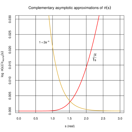
Function $\vartheta(s)$ has two simple asymptotic regimes for real and positive $s$, as can be seen from the functional equation (26):

$$\vartheta(s)\xrightarrow{s\to 0}\sqrt{\frac{\pi}{s}}\quad\text{and}\quad\vartheta(s)\xrightarrow{s\to\infty}1+2e^{-s}\,.$$ (32)

We can visualize these asymptotes by plotting the logarithm of the quotient between $\vartheta$ and each of them. This is done in figure 1, where we can see that the limit $s\to 0$ is (reasonably) valid for $s<1$ and the limit $s\to\infty$ is valid for $s>2$. In the middle regime $s\in[1,2]$ none of the two former cases is accurate enough, and we will have a mixed, interpolating regime between them.

Figure 1: Complementary asymptotic regimes of the $\vartheta$ function. Logarithms of the quotient of $\vartheta$ and its asymptotes are shown. A good approximation can be seen as a flat line at zero height. Both regimes cross near $1.5$, which is the center of the interval $[1,2]$ where the accuracy is lower. Note that the horizontal line at 0.01 signals that the quotient is 1% different from 1. All plots in this paper were done using R [25].

The first case we will consider is $s\to 0$. In this regime, we simply make the integration contour $\gamma$ pass near the origin in the complex plane, where $\vartheta$ has a singularity. Assuming that the main contribution to the integral will come from this region, we can replace $\vartheta$ by its asymptotic value when $s\to 0$ and write

$$\omega_{J}(r)\approx\frac{2r}{2\pi i}\int_{\gamma}e^{sr^{2}}\Biggl{[}\prod_{j=1}^{J}\sqrt{\frac{\pi}{q_{j}^{2}s}}\Biggr{]}\,{\rm d}s\,.$$ (33)

This integral is an elementary inverse Laplace transform:

$$\omega_{J}(r)\approx\frac{\pi^{\frac{J}{2}}}{\operatorname{vol}Q}\,\frac{2r}{2\pi i}\int_{\gamma}e^{sr^{2}}\frac{\,{\rm d}s}{s^{\frac{J}{2}}}=\frac{2\pi^{\frac{J}{2}}}{\Gamma(\frac{J}{2})}\,\frac{r^{J-1}}{\operatorname{vol}Q}\,.$$ (34)

Equation (34) is the derivative of (7), that is, BP count. It is valid for large $r$ distances, because it has been obtained using small $s$ region (note that a well known property of Laplace transform pairs is that the asymptotic behaviour of a signal for large $r$ is determined by the small $s$ behaviour of its transform and vice versa). For this reason we call the formula (34) the large distance regime, or BP regime.

But we can make the restriction imposed on the distance more quantitative in the following way. The best choice for the real part of the contour is the saddle point of integral (34), which is the stationary point of the function

$$\phi(s)=sr^{2}-\frac{J}{2}\,\log s\,.$$ (35)

This saddle point is

$$s^{*}=\frac{J}{2r^{2}}\,,$$ (36)

and in its vicinity we find the most important contribution to the integral. But the replacement of the $\vartheta(s)$ functions by its small-$s$ behavior is valid only if the argument $s$ is less than 1 (see figure 1), so we must have

$$s^{*}q_{j}^{2}=\frac{Jq_{j}^{2}}{2r^{2}}<1\quad\text{for all $j$}\,.$$ (37)

Nevertheless, condition (37) does not guarantee the validity of the replacement $\vartheta(s)\to\sqrt{\frac{\pi}{s}}$ on the integration contour away from the real axis. A stronger restriction is imposed by demanding the applicability of the saddle point method in this regime. If the steepest descent approximation is valid, then the main contribution to the integral comes from the vicinity of the saddle point, which justifies the replacement of the asymptote. The exact and approximate evaluations of (34) will have the same validity if both methods reach the same result. But the saddle point approximation on (34) has the effect of using Stirling’s approximation on the gamma function. Thus, both methods agree if $J$ is large enough.

The correctness of the saddle point approximation of (34) can be assessed by rewriting it in the form

$$\omega_{J}(r)\approx\pi^{\frac{J}{2}}\,\frac{2r}{2\pi i}\int_{\gamma}e^{sr^{2}-\frac{J}{2}\log(q^{2}s)}\,{\rm d}s\quad\text{with }\log q=\frac{1}{J}\sum^{J}_{i=1}\log q_{i}\,.$$ (38)

The change of variable $q^{2}s=w$ transforms the exponent $\phi$ of the integrand into

$$\phi(w)=J\Bigl{[}\frac{w}{h}-\frac{1}{2}\log w\Bigr{]}\,,$$ (39)

where $h=\frac{Jq^{2}}{r^{2}}$. The validity condition of the saddle point approximation is $\phi(w^{*})\gg 1$ with $w^{*}=h/2$ the stationary point of $\phi$. This condition is fulfilled if $J$ is large and

$$\frac{w^{*}}{h}-\frac{1}{2}\log w^{*}=\frac{1}{2}\Bigl{(}1-\log\frac{h}{2}\Bigr{)}>1\quad\Rightarrow\quad h<\frac{2}{e}\approx 0.736\,,$$ (40)

which is analogous to the condition stated by Bousso and Polchinski for the validity of their formula. We have derived it as a validity condition for the small-$s$ asymptotic regime of the exact counting formula.

Finally, the large $J$ condition controls the validity of Stirling’s approximation for the gamma function. But this restriction is not needed because the integral has been done in closed form. Thus, only condition (40) remains.

2.3 The small distance regime

In this case we are in the regime in which the asymptotic expansion of $\vartheta$ for large values of its argument is valid. We can write $\Omega_{J}(r)$ in (29) as

$$\Omega_{J}(r)=1+\frac{1}{2\pi i}\int_{\gamma}f(s)e^{\phi(s)}\,{\rm d}s\,,\quad\text{with}\quad\begin{cases}f(s)=\frac{1-e^{-sr^{2}}}{s}\,,\\ \phi(s)=sr^{2}+\sum^{J}_{i=1}\log\bigl{(}1+2e^{-q_{i}^{2}s}\bigr{)}\,.\end{cases}$$ (41)

The saddle-point approximation to this integral is given by

$$\Omega_{J}(r)\approx 1+\frac{1}{2\pi i}\,if(s^{*})e^{\phi(s^{*})}\sqrt{\frac{2\pi}{\phi^{\prime\prime}(s^{*})}}\,,$$ (42)

where $s^{*}$ is the stationary point of $\phi(s)$. The saddle point $s^{*}$ is a minimum for real $s$; hence, the steepest descent contour crosses vertically the real axis and coincides locally with $\gamma$. Unfortunately, we cannot solve the saddle point equation in closed form for arbitrary charges. Nevertheless, in the simplest case in which all charges are equal $q_{1}=\cdots=q_{J}=q$, we obtain

$$r^{2}=\frac{2Jq^{2}}{e^{s^{*}q^{2}}+2}\quad\Rightarrow\quad s^{*}q^{2}=\log 2\Bigl{(}\frac{Jq^{2}}{r^{2}}-1\Bigr{)}\,.$$ (43)

The saddle point computed through (43) is consistent with the regime of large argument of $\vartheta$ if

$$s^{*}q^{2}=\log 2\Bigl{(}\frac{Jq^{2}}{r^{2}}-1\Bigr{)}>2\quad\Rightarrow\quad\frac{Jq^{2}}{r^{2}}>1+\frac{e^{2}}{2}\approx 4.694\,.$$ (44)

This condition is satisfied for fixed charge $q$ and dimension $J$ if the distance is small enough; for this reason this regime is called the small distance regime.

In terms of the parameter $h=\frac{Jq^{2}}{r^{2}}$, the approximate saddle point (which will be called $u(h)=q^{2}s^{*}(h)$) is, gluing together eqs. (37, 43)

$$u(h)=q^{2}s^{*}(h)=\begin{cases}\frac{1}{2}h&\text{if $h<2$,}\\ \log 2(h-1)&\text{if $h>5$.}\end{cases}$$ (45)

Eq. (45) is plotted in figure 2, along with the numerical solution obtained in a range of $h$ which is not covered so far, but will be considered in the next subsection.

Figure 2: Numerical saddle point $u(h)$ of the $\omega_{J}(r)$ integrand for equal charges. For $h<2$ it agrees with its low-$h$ asymptote, and for $h>5$ it agrees with its high-$h$ asymptote. The mixed regime, where the numerical solution smoothly interpolates between the asymptotes, is shown in the central rectangle.

Substituting the large $h$ regime for $u(h)$ leads to

$$\begin{split}\phi(s^{*})&=\frac{r^{2}}{q^{2}}\,u(h)+J\log\bigl{(}1+2e^{-u(h)}\bigr{)}=J\Bigl{[}\frac{\log 2(h-1)}{h}+\log\Bigl{(}\frac{h}{h-1}\Bigr{)}\Bigr{]}\,,\\ \phi^{\prime\prime}(s^{*})&=\frac{2Jq^{4}e^{-u(h)}}{(1+2e^{-u(h)})^{2}}=Jq^{4}\Bigl{(}\frac{h-1}{h}\Bigr{)}\,,\\ f(s^{*})&=q^{2}\frac{1-e^{-\frac{Ju(h)}{h}}}{u(h)}=q^{2}\frac{1-e^{-J\frac{\log 2(h-1)}{h}}}{\log 2(h-1)}\,,\end{split}$$ (46)

and the saddle-point approximations for $\Omega_{J}(r)$ and $\omega_{J}(r)$ result in

$$\Omega_{J}(r) =1+\frac{1}{\sqrt{2\pi J}}\,\frac{(2h-2)^{\frac{J}{h}}-1}{\log(2h-2)}\,\Bigl{(}\frac{h}{h-1}\Bigr{)}^{J+\frac{1}{2}}\,,$$ (47a)

$$\omega_{J}(r) =\frac{(2h-2)^{\frac{J}{h}}}{q\sqrt{2\pi h}}\Bigl{(}\frac{h}{h-1}\Bigr{)}^{J+\frac{1}{2}}\,.$$ (47b)

We must note that these magnitudes depend on $r$ through $h=\frac{Jq^{2}}{r^{2}}$. It should be stressed that (47b) has been obtained by using the saddle point approximation of (27) and not by differentiating (47a); although these two results are asymptotically equivalent, they differ in subleading terms.

We will now consider the validity of formulae (47a, 47b). The saddle-point approximation is good if $\phi(s^{*})\gg 1$. We could rewrite $\phi(s^{*})$ as follows:

$$\phi(s^{*})=J\psi(h)\quad\text{with}\quad\psi(h)=\frac{\log 2(h-1)}{h}+\log\Bigl{(}\frac{h}{h-1}\Bigr{)}\,,$$ (48)

and, for large $J$, demand $\psi(h)>1$ as we did before. But this would contradict (44), so we better choose some $J_{0}>2$ and write

$$\phi(s^{*})=\frac{J}{J_{0}}J_{0}\psi(h)\,,$$ (49)

which satisfies $\phi(s^{*})\gg 1$ if $J/J_{0}$ is large and $J_{0}\psi(h)>1$. For example, we have

$$J_{0}=\{1,2,3,4,5\}\quad\Rightarrow\quad h<\{2.2,7.2,12.5,18.3,24.3,30.6\}\,.$$ (50)

This restriction implies that the distance cannot be too small in order to preserve the validity of the saddle-point approximation.

For very small $r$, we can choose a large real part of $s$ and approximate $(1+2e^{-q^{2}s})^{J}\approx 1+2Je^{-q^{2}s}$, and then $\Omega_{J}(r)$ is reduced to

$$\Omega_{J}(r)\xrightarrow{r\to 0}\theta(r^{2})+2J\theta(r^{2}-q^{2})\,,$$ (51)

that is, only the node at the origin and its $2J$ neighbors contribute to $\Omega_{J}$. The formula (47a) cannot reproduce this result, and therefore there must exist a validity condition which forbids too small distances. This is exemplified in (50). However, that restriction turns out to be of no importance because close-to-the-origin nodes represent a negligible fraction of the whole.

2.4 The middle distance regime

When $h$ takes a value in which no accurate asymptotic approximation of $\vartheta$ is available, we are in the middle distance or crossing regime. In this situation the saddle point can be computed only numerically. This has been done in figure 2 by solving the following equation

$$-\frac{\vartheta^{\prime}(w)}{\vartheta(w)}=\frac{1}{h}\,,$$ (52)

whose solution $u(h)$ is the saddle point. This solution can always be obtained, with no condition on the value of $h$, but it coincides with (45) in the specified ranges. Using this solution, the saddle-point approximation of $\omega_{J}(r)$ can be computed, but only for large $J$, and only for not too small distances.

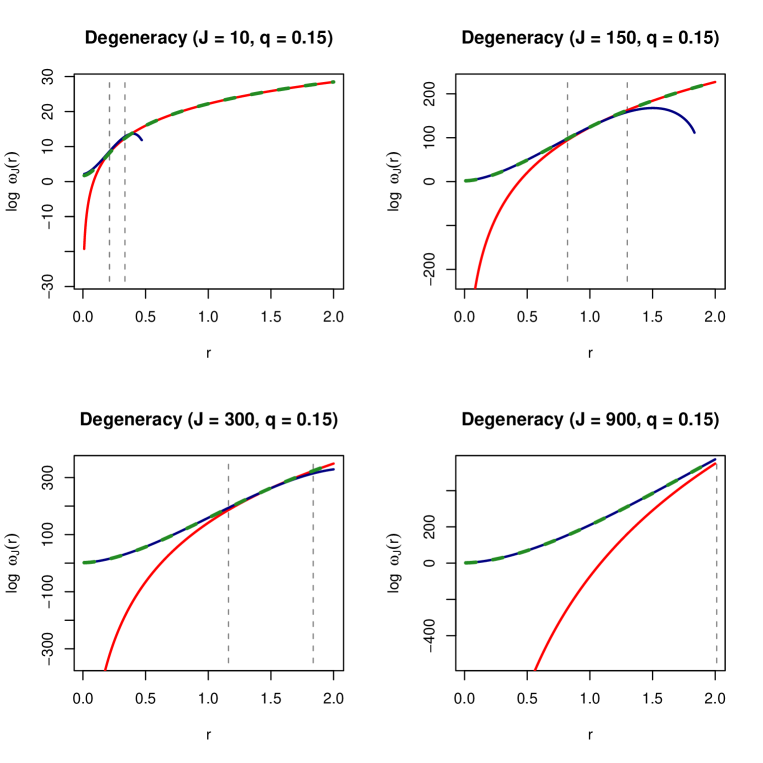
In figure 3, we compare equations (34) and (47b), displaying between them the crossing regime. Both small and large distance regimes show up for constant $J$ and $q$ at different distances $r$. Note that small $h$ corresponds to large $r$ and vice versa, but “small” and “large” distances are $J$-dependent concepts, so that both regimes can have their own range of validity. Moreover, for sufficiently high $J$ almost all relevant distances in flux space can be considered “small”. In such cases, the BP formula (7,34) should be replaced by the correct asymptotic one given in (47a,47b).

Figure 3: Asymptotic regimes of the Landscape degeneracy $\omega_{J}(r)$ for equal charges $q=0.15$ and different $J$ as functions of $r$. The actual $\omega_{J}(r)$ is close to the upper envelope of both curves (green dashed line). For small $J$ the large distance or BP regime dominates (red line), but for large $J$ the small distance regime (blue line) spans the whole $[0,2]$ interval. Vertical dashed lines delimit the crossing regime, corresponding to $h\in[2,5]$, which is above $r=2$ in the $J=900$ panel.

In the case of different charges in the small distance regime, the approximate saddle-point equation cannot be exactly solved. Thus, one needs to solve the complete saddle-point equation

$$r^{2}+\sum^{J}_{j=1}q_{j}^{2}\,\frac{\vartheta^{\prime}(q_{j}^{2}s)}{\vartheta(q_{j}^{2}s)}=0\,.$$ (53)

The $h$ parameter does not appear in this equation, and it is not clear what kind of average charge must be used to define it.

However, there is a class of models in which the crossing regime dominates over the small and large distance regimes. It is enough to consider a charge distribution in which the smallest and biggest charges are well separated. In such cases, there will be regions in the $s$ plane where every $\vartheta$ factor could in principle lie in a different asymptotic regime, and thus we will obtain a plethora of intermediate regimes in which neither BP nor small distance regimes will be accurate enough. For large $J$, the degeneracy density $\omega_{J}(r)$ can be obtained by computing the numerical solution of (52) and then using it in the saddle point approximation of the exact integral (27).

3 Applications

In this section, we will show how $\omega_{J}(r)$ helps to estimate other properties of BP models. We will consider the number of states in the anthropic window, the distribution of non-vanishing fluxes of a typical state, the minimum cosmological constant and a possible consequence on the KKLT moduli stabilization mechanism.

3.1 Number of states in the Weinberg Window

The number of states of positive cosmological constant bounded by a small value $\Lambda_{\varepsilon}$ is the number of nodes of the lattice in flux space whose distance to the origin lies in the interval $[R_{0},R_{\varepsilon}]$, where $R_{0}=\sqrt{2|\Lambda_{0}|}$ and $R_{\varepsilon}=\sqrt{2(\Lambda_{\varepsilon}-\Lambda_{0})}\approx R_{0}+\frac{\Lambda_{\varepsilon}}{R_{0}}$ so that the width of the shell is $\varepsilon=\frac{\Lambda_{\varepsilon}}{R_{0}}$:

$$\mathcal{N}_{\varepsilon}=\Omega_{J}(R_{\varepsilon})-\Omega_{J}(R_{0})\approx\omega_{J}(R_{0})\frac{\Lambda_{\varepsilon}}{R_{0}}\,.$$ (54)

We remind the reader that $\Omega_{J}(r)$ is the number of states inside a sphere of radius $r$ in flux space and $\omega_{J}(r)=\frac{\partial\Omega_{J}(r)}{\partial r}$. If $\Lambda_{\varepsilon}$ is the width of the anthropic range $\Lambda_{\text{WW}}$ (the so-called Weinberg Window), then the number of states in it is

$$\mathcal{N}_{\text{WW}}=\frac{\omega_{J}(R_{0})}{R_{0}}\Lambda_{\text{WW}}\,.$$ (55)

Computation of $\omega_{J}(R_{0})$ should be done along the lines of the previous section. Thus, the expression (55) can be used for all values of $h$ using the relevant approximation of the exact formula (27), which includes the BP regime as well as the small distance and crossing regimes.

3.2 Typical number of non-vanishing fluxes

As before, consider the nodes of the lattice $\mathcal{L}$ having cosmological constant between 0 and $\Lambda_{\varepsilon}$. They will lie inside a thin shell of width $\varepsilon=R_{\varepsilon}-R$ above radius $R$ (former radius $R_{0}$ will be called $R$ in this section). The set of nodes inside the shell will be called $\Sigma_{\varepsilon}$:

$$\Sigma_{\varepsilon}=\bigl{\{}\lambda\in\mathcal{L}\colon R\leq\|\lambda\|\leq R_{\varepsilon}\bigr{\}}\quad\text{\quad}\bigl{|}\Sigma_{\varepsilon}\bigr{|}=\mathcal{N}_{\varepsilon}\,.$$ (56)

We will assume that $\varepsilon$ is smaller than the charges $q_{i}$ so that (54) is valid but $\mathcal{N}_{\varepsilon}\gg 1$.

Taking $J=2$, we will find at most four nodes in the shell with one vanishing component. Thus, the remaining states will have two nonzero components. In the $J=3$ case, the states in the shell are located at the axes (at most six) with only one nonzero component, at the coordinate planes with two nonzero components (a larger charge-dependent number) and at the “bulk” of the sphere with all three nonzero components (the most abundant). In this way, we find that the typical number of non-vanishing components is $J$ for the cases $J=2,3$.

Thus, after drawing a node of the shell at random (assuming that all nodes have the same chances of being selected), the probability of all fluxes being different from zero will be very high. In this section we wonder whether it happens for all $J$.

We will answer this question by computing the fraction of states in the shell having a fixed number $j$ of non-vanishing components. If all states are equiprobable, the quotient between this number and the total number of nodes in the shell will yield the probability distribution of the values $j$ taking into account only abundances of states.

We can expect this probability distribution to have a peak at certain value $j^{*}$. This $j^{*}$ will be taken as the typical number of non-vanishing fluxes of the states in the shell. For small values of $J$ we know that $j^{*}=J$. We will see that this is not true for sufficiently high $J$.

We will now outline the calculation and give the results. The details can be found in appendix A.

For any state $\lambda\in\Sigma_{\varepsilon}$ having exactly $j$ non-vanishing components, we define $\alpha=\frac{j}{J}$. When $\lambda$ is selected at random from $\Sigma_{\varepsilon}$ with uniform probability, $\alpha$ becomes a discrete random variable taking values in the $[0,1]$ interval whose probability distribution is given by

$$P(\alpha)=\frac{\mathcal{N}_{\varepsilon}(j)}{\mathcal{N}_{\varepsilon}}\,,$$ (57)

where $\mathcal{N}_{\varepsilon}(j)$ is the number of nodes in the shell $\Sigma_{\varepsilon}$ having exactly $j$ non-vanishing components. The formula (57) takes into account only the abundances of states in the shell, and hence we are assuming that all states in $\Sigma_{\varepsilon}$ are equally probable.

Computation of the quantity $\mathcal{N}_{\varepsilon}(j)$ can be achieved using the principle of inclusion-exclusion. For simplicity, we will assume equal charges $q_{1}=\cdots=q_{J}=q$. In the general expression (102) we substitute the number of nodes in the shell (54) and the exact density of states (27), obtaining (107). After normalization, it results in the following exact representation for the probability distribution (see (108) in appendix A):

$$P(\alpha)=\frac{2R}{\omega_{J}(R)}\binom{J}{\alpha J}\frac{1}{2\pi i}\int_{\gamma}e^{\phi(s,\alpha)}\,{\rm d}s\quad\text{with}\quad\phi(s,\alpha)=sR^{2}+\alpha J\log\bigl{[}\vartheta(q^{2}s)-1\bigr{]}\,.$$ (58)

With the assumptions made, we find that $P(\alpha)$ depends on the radius of the $\Lambda=0$ sphere but it is independent of $\varepsilon$. The same method can be used for analyzing the distribution $P(\alpha)$ over the whole Landscape, that is, inside the sphere of radius $R_{1}$. The resulting expression and the subsequent analysis are analogous, and the result is quite similar; in appendix B the calculation is carried out in the BP regime.

Using the saddle-point method again, we can approximate the exact formula (58) by (see (115) in appendix A)

$$P(\alpha)\propto e^{Js(\alpha)}\quad\text{with}\quad s(\alpha)=-\alpha\log\alpha-(1-\alpha)\log(1-\alpha)+\frac{1}{J}\phi(\upsilon,\alpha)\,,$$ (59)

where $\upsilon=q^{2}s^{*}$, and $s^{*}$ is the stationary point of the function $\phi(s,\alpha)$ defined in (58). The saddle point $\upsilon$ is a function of a single variable $h\alpha$ with $h=\frac{Jq^{2}}{R^{2}}$, and it has two well-defined asymptotic regimes and a crossing regime which requires numerical computation. This is plotted in appendix A, figure 9.

The distribution (59) has a pronounced peak located at $\alpha^{*}(h)$. This is the typical number of non-vanishing fluxes in the shell $\Sigma_{\epsilon}$ (and essentially also in the whole Landscape). Its computation must be done numerically by solving the following equation (see (117) in appendix A):

$$\vartheta\bigl{[}\upsilon(h\alpha)\bigr{]}=\frac{1}{1-\alpha}\,.$$ (60)

For each positive value of $h$, (60) has a unique solution $\alpha^{*}(h)$ with its own regimes, which is plotted in figure 4.

Figure 4: (Left) Numerical solution $\alpha^{*}(h)$ along with its asymptotic regimes shown in equations (119) (small $h$) and (121) (large $h$). The dashed line is the curve $\alpha^{*}=\frac{1}{h}$. (Right) Samples of the typical number of non-vanishing fluxes. The two sampling methods described in the text have been used: The inside-shell, maximum-frequency method (blue hollow circles) and the inside-ball, average-frequency method (green bullets). The saddle point solution displayed in the left panel is also shown (red line).

Thus, $P(\alpha)$ is locally Gaussian around its peak,

$$\log P(\alpha)\approx\log P(\alpha^{*})-\frac{1}{2}J|s^{\prime\prime}(\alpha^{*})|(\alpha-\alpha^{*})^{2}\,,$$ (61)

with standard deviation

$$\frac{1}{\sqrt{J|s^{\prime\prime}(\alpha^{*})|}}=\sqrt{\frac{\alpha^{*}(1-\alpha^{*})}{J}}\leq\frac{1}{2\sqrt{J}}\,.$$ (62)

Therefore, for large $J$ the peak at $\alpha^{*}$ is very narrow. We can conclude that an overwhelming fraction of states in the shell (and in the whole Landscape) have $J\alpha^{*}$ non-vanishing fluxes, and that for high dimensions this typical number is far from $J$, which is the typical value for the low-dimensional case considered at the beginning of this subsection.

We should emphasize that the calculation outlined here uses the saddle-point approximation, and therefore it is not valid for small $J$.

Numerical searches have been carried out varying $J$ for constant $q$ and $R$, estimating $\alpha^{*}(h)$ by counting states. Results are shown in figure 4 versus the saddle point curve described above. Two sampling methods have been used:

• The inside-shell, maximum-frequency method samples states inside a shell and computes the typical number of non-vanishing fluxes as the value of maximum frequency. Some advantages can be mentioned, such as the possibility of performing a better sampling of the true set we are describing, but also some disadvantages: the size of the sample is smaller, there is an unavoidable intrusion of exterior secant states in the shell [23, 24], and the sample shows a stronger dependence with the details of the lattice.

• The inside-ball, average-frequency method samples states inside a ball and computes the typical number of non-vanishing fluxes using the average frequency. When compared with the previous method, this method has the disadvantage of sampling mostly secant states, but it has the advantage of accounting for bigger sample sizes. It also averages over the lattice details, giving a satisfactory agreement with the saddle point computation.

Data used in both samples are a shell of radius $R=\sqrt{2}$ and width $\frac{q}{2}$ with $q=0.15$, and dimensions $J$ between 2 and 200 in the first method and between 2 and 275 in the second. In both cases, the $h$ parameter has been computed using averaged distances, and the lattice details can be observed in the first sample in the form of a jagged curve. Note that for dimensions up to 7 the typical number of non-vanishing fluxes is $J$ (that is, $\alpha^{*}=1$) but this abruptly changes to fit the saddle point curve.

We will close this section with two remarks. First, as the different sampling methods considered above suggest, $\alpha^{*}(h)$ curve is very robust as a property of the BP Landscape, in the sense that generic subsets of the lattice have $\alpha^{*}(h)$ curves which differ only in subleading terms. We can see an example of this feature in appendix B. And finally, the role played by the exact formula (27) for $\omega_{J}(r)$ in the computation of $P(\alpha)$ is essential: replacing it with the BP estimate (the “pure BP regime”) results in a probability distribution valid only for $h<\frac{8\pi}{27}$ with the same typical fraction $\alpha^{*}(h)$. Details of this calculation are given in appendix B.

3.3 Estimating the minimum positive cosmological constant

In this subsection we will estimate the explicit dependence of the minimum positive cosmological constant with respect to the parameters of the Landscape. We will call $\Lambda^{*}$ the actual minimum value, and $\Lambda_{\varepsilon}$ the corresponding estimator. We will assume that all charges are equal, for simplicity. In this case, we have

$$\Lambda^{*}=\Lambda_{0}+\frac{q^{2}}{2}\underbrace{\sum^{J}_{i=1}n_{i}^{2}}_{N}\,,$$ (63)

and we should choose the smallest integer $N$ satisfying two conditions: it should yield $\Lambda^{*}\geq 0$, and it should be representable as a sum of $J$ integer squares. If we call such a number $N_{J}(q)$, we have the exact formula

$$\Lambda^{*}=\Lambda_{0}+\frac{q^{2}}{2}\,N_{J}(q)\,.$$ (64)

The computation of $N_{J}(q)$ can be avoided as we change it by another integer $N$ satisfying only the first condition:

$$\Lambda_{0}+\frac{q^{2}N}{2}\geq 0\quad\text{but}\quad\Lambda_{0}+\frac{q^{2}(N-1)}{2}<0\,,$$ (65)

that is,

$$\frac{2|\Lambda_{0}|}{q^{2}}\leq N<\frac{2|\Lambda_{0}|}{q^{2}}+1\,.$$ (66)

Thus, $N$ is the smallest integer greater than or equal to $\frac{2|\Lambda_{0}|}{q^{2}}$, also called ceiling:

$$N=\biggl{\lceil}\frac{2|\Lambda_{0}|}{q^{2}}\biggr{\rceil}\,.$$ (67)

If $N$ is decomposable as the sum of $J$ squares, we have $N_{J}(q)=N$, but in general the inequality

$$\biggl{\lceil}\frac{2|\Lambda_{0}|}{q^{2}}\biggr{\rceil}\leq N_{J}(q)$$ (68)

holds. So we have a lower bound for the minimum value of the cosmological constant, and this is our estimator:

$$\Lambda^{*}\geq\Lambda_{\varepsilon}=\Lambda_{0}+\frac{q^{2}}{2}\biggl{\lceil}\frac{2|\Lambda_{0}|}{q^{2}}\biggr{\rceil}\,.$$ (69)

It should be noted that this lower bound is independent of $J$, even though we can expect it to work better when the error for the replacement is small, that is, for large $J$. In figure 5 we show the lower bound along with the actual, brute-force computed minimum, and we find a very good agreement for $J=4$ and greater. In the figure we can see a straight upper envelope of the lower bound, which can be obtained by noting that $\lceil x\rceil<1+x$, and thus $\Lambda_{0}+\frac{q^{2}}{2}\bigl{\lceil}\frac{2|\Lambda_{0}|}{q^{2}}\bigr{\rceil}<\frac{q^{2}}{2}$.

Figure 5: Actual brute-force computation of the minimum positive cosmological constant for equal charges in $J=2,3,4$ (hollow circles), along with the lower bound given in (69) versus charge values. The agreement is almost complete for $J=4$, and therefore for greater $J$ as well.

Generalizing the preceding argument is not easy, because for different charges we have

$$\Lambda=\Lambda_{0}+\frac{q^{2}}{2}\sum^{J}_{i=1}\frac{q_{i}^{2}}{q^{2}}\,n_{i}^{2}\,,$$ (70)

where $q$ is some average value of the charges. The sum in (70) is not an integer, and its possible values near $\Lambda=0$ depend strongly on the particular charge values.

We also lack a reasonable upper bound for the minimum value, because the replacement of $N_{J}(q)$ by $N_{J}(q)+1$ in (65) gives a window of width $\frac{q^{2}}{2}$. The corresponding distance in flux space is of the order of the cell spacing, which is too big to be a good upper bound.

We will adopt another approach from now on. Our strategy will consist of computing the number of states of cosmological constant between 0 and $\Lambda_{\varepsilon}$ and equate it to the degeneracy of the minimum positive $\Lambda$ states computed in a different way.

Let $\lambda^{*}$ be a minimum cosmological constant state, that is, $\Lambda(\lambda^{*})=\Lambda^{*}$. There are other valid minima of equal value $\Lambda^{*}$. Some of them can be derived from $\lambda^{*}$ using lattice symmetries, but there will be a set of minima which cannot be related by any symmetries. We will call the set of minima modulo lattice symmetries $\Sigma^{*}$, and its cardinality $|\Sigma^{*}|$ the essential degeneracy. For small $J$, $\Sigma^{*}$ can contain only one state, but we can expect $\Sigma^{*}$ to grow with $J$.

Consider a state $\lambda^{*}=q(n_{1}^{*},\cdots,n_{J}^{*})$ in $\Sigma^{*}$, and let $f_{k}(\lambda^{*})$ be the frequency of the non-negative number $k$ in the sequence $|n_{1}^{*}|,\cdots,|n_{J}^{*}|$. Note that $\sum_{k=0}^{\infty}f_{k}=J$, and the number of different nodes in $\mathcal{L}$ that can be derived from $\lambda^{*}$ using the lattice symmetries is

$$\frac{J!\,2^{J-f_{0}}}{\prod_{k=0}^{\infty}f_{k}!}\,.$$ (71)

The rationale behind equation (71) is to count permutations of the $J$ components except for the components which have the same absolute value, and multiply them by the number of different “$J$-quadrants” which can contain such a state (different signs of its components), which depend on the number $J-f_{0}$ of non-vanishing components.

Of course, knowing the sequence $\{f_{k}\}_{k=0,\cdots,\infty}$ is equivalent to knowing the exact state $\lambda^{*}$, which is a very difficult problem for large $J$. So we can bound the true value of the degeneracy (71) between the two extreme cases of states having different values in all non-vanishing components (and then, all values are non-degenerate except 0, $f_{k}=1$ if $k\neq 0$) and states having all non-vanishing components equal (and then, all frequencies vanish $f_{k}=0$ except for two values $k\in\{0,\ell\}$ for some $\ell$). Then, taking the same number of null components $f_{0}$,

$$\frac{J!\,2^{J-f_{0}}}{f_{0}!\,(J-f_{0})!}\leq\frac{J!\,2^{J-f_{0}}}{\prod_{k=0}^{\infty}f_{k}!}\leq\frac{J!\,2^{J-f_{0}}}{f_{0}!}\,.$$ (72)

The degeneracy of the minimum $\Lambda^{*}$ is obtained by adding all degeneracies of the different states $\lambda^{*}\in\Sigma^{*}$, and thus we obtain the bound:

$$\sum_{\lambda^{*}\in\Sigma^{*}}\frac{J!\,2^{J-f_{0}(\lambda^{*})}}{f_{0}(\lambda^{*})!\,(J-f_{0}(\lambda^{*}))!}\leq\sum_{\lambda^{*}\in\Sigma^{*}}\frac{J!\,2^{J-f_{0}(\lambda^{*})}}{\prod_{k=0}^{\infty}f_{k}(\lambda^{*})!}\leq\sum_{\lambda^{*}\in\Sigma^{*}}\frac{J!\,2^{J-f_{0}(\lambda^{*})}}{f_{0}(\lambda^{*})!}\,.$$ (73)

Equating the degeneracy (middle term of (73)) to the number of states in the shell (55), we have

$$\frac{R}{\omega_{J}(R)}\,\sum_{\lambda^{*}\in\Sigma^{*}}\frac{J!\,2^{J-f_{0}(\lambda^{*})}}{f_{0}(\lambda^{*})!\,(J-f_{0}(\lambda^{*}))!}\leq\Lambda_{\varepsilon}\leq\frac{R}{\omega_{J}(R)}\,\sum_{\lambda^{*}\in\Sigma^{*}}\frac{J!\,2^{J-f_{0}(\lambda^{*})}}{f_{0}(\lambda^{*})!}\,.$$ (74)

Note that the shell’s width is taken as $\Lambda_{\varepsilon}$ in (74) instead of $\Lambda^{*}$, because the number of states in the shell is an estimate. Therefore, (74) can be taken as a definition of the minimum estimator $\Lambda_{\varepsilon}$.

So we are faced with estimating $f_{0}(\lambda^{*})$, or equivalently, the fraction of non-vanishing components $\alpha(\lambda^{*})=\frac{J-f_{0}(\lambda^{*})}{J}$, in terms of which

$$\frac{R}{\omega_{J}(R)}\,\sum_{\lambda^{*}\in\Sigma^{*}}\frac{J!\,2^{J\alpha(\lambda^{*})}}{[J\alpha(\lambda^{*})]!\,[J(1-\alpha(\lambda^{*}))]!}\leq\Lambda_{\varepsilon}\leq\frac{R}{\omega_{J}(R)}\,\sum_{\lambda^{*}\in\Sigma^{*}}\frac{J!\,2^{J\alpha(\lambda^{*})}}{[J(1-\alpha(\lambda^{*}))]!}\,.$$ (75)

The sum extended to $\Sigma^{*}$ can be replaced by averaging over a probability measure of $\alpha$ restricted to $\Sigma^{*}$:

$$\frac{R|\Sigma^{*}|}{\omega_{J}(R)}\,\int_{0}^{1}\frac{J!\,2^{J\alpha}}{[J\alpha]!\,[J(1-\alpha)]!}\,{\rm d}P(\alpha|\Sigma^{*})\leq\Lambda_{\varepsilon}\leq\frac{R|\Sigma^{*}|}{\omega_{J}(R)}\,\int_{0}^{1}\frac{J!\,2^{J\alpha}}{[J(1-\alpha)]!}\,{\rm d}P(\alpha|\Sigma^{*})\,.$$ (76)

The conditional distribution $P(\alpha|\Sigma^{*})$ is not known, because the set $\Sigma^{*}$ is very difficult to enumerate. We must assume the robustness of the distribution $P(\alpha)$ computed in the previous subsection, and approximate $P(\alpha|\Sigma^{*})\approx P(\alpha)$. We then use the Gaussian nature of $P(\alpha)$ for large $J$, and we perform the average simply by taking the most probable value:

$$\frac{R|\Sigma^{*}|}{\omega_{J}(R)}\,\frac{J!\,2^{J\alpha^{*}}}{[J\alpha^{*}]!\,[J(1-\alpha^{*})]!}\leq\Lambda_{\varepsilon}\leq\frac{R|\Sigma^{*}|}{\omega_{J}(R)}\,\frac{J!\,2^{J\alpha^{*}}}{[J(1-\alpha^{*})]!}\,.$$ (77)

This equation is not useful because we lack an estimate for $|\Sigma^{*}|$. Nevertheless, for equal charges we can replace $\Lambda_{\varepsilon}$ with (69) and use (77) to obtain a lower bound for the essential degeneracy $|\Sigma^{*}|$:

$$|\Sigma^{*}|\geq\frac{\omega_{J}(R)}{R}\,\frac{[J(1-\alpha^{*})]!}{J!\,2^{J\alpha^{*}}}\biggl{(}\Lambda_{0}+\frac{q^{2}}{2}\biggl{\lceil}\frac{2|\Lambda_{0}|}{q^{2}}\biggr{\rceil}\biggr{)}\,.$$ (78)

Thus, for the special case of equal charges, we have estimates for the minimum value of the cosmological constant and for its essential degeneracy. Figure 6 compares the estimate given in (78) with actual brute-force computations for low $J$.

Figure 6: Actual brute-force computation of the essential degeneracy $|\Sigma^{*}|$ of the minimum positive cosmological constant states for equal charges in $J=3,4$ (circles) along the lower bound given in (78) (thin lines) versus charge values. The strong oscillations of the lower bound are caused by the ceiling function (note logarithmic scale). Thick lines are obtained replacing the lower bound of $\Lambda_{\varepsilon}$ by its upper envelope, and they represent an average asymptotic regime which is better followed in the $J=4$ sample.

As said above, generalizing (69) to the case of distinct charges is difficult. Nevertheless, we can assume that for charges not only distinct but incommensurate, the essential degeneracy will be $|\Sigma^{*}|=1$. Furthermore, the symmetry degeneracy is reduced to $2^{J\alpha}$, so that we have the estimate

$$\Lambda_{\varepsilon}\approx\frac{2^{J\alpha^{*}}R}{\omega_{J}(R)}\,.$$ (79)

Note that this formula is equivalent to the number of states in the Weinberg Window, (55), where $\mathcal{N}_{\text{WW}}$ should be replaced by the symmetry degeneracy and solved for the width $\Lambda_{\varepsilon}$. But we can improve this by replacing the degeneracy $2^{J\alpha^{*}}$ by its mean value computed using the Gaussian distribution $P(\alpha)$ given in formulae (61) and (62):

$$\langle 2^{J\alpha}\rangle_{P(\alpha)}=\int_{0}^{1}2^{J\alpha}\,{\rm d}P(\alpha)\approx\int_{\mathbb{R}}2^{J\alpha}e^{-\frac{J(\alpha-\alpha^{*})}{2\alpha^{*}(1-\alpha^{*})}}\frac{\sqrt{J}\,{\rm d}\alpha}{\sqrt{2\pi\alpha^{*}(1-\alpha^{*})}}=2^{J\alpha^{*}[1+\frac{\log 2}{2}(1-\alpha^{*})]}\,.$$ (80)

We can check this estimate with the brute-force data for low $J$ (and thus $\alpha^{*}=1$) by choosing charges with constant geometric mean. In the BP regime $\omega_{J}(R)$ depends only on the geometric mean and therefore it does not fluctuate. Figure 7 shows that (79) is a good estimator for the mean value of such fluctuations.

Figure 7: Each box plot represents a sample of 100 choices of $J$ charges with constant geometric average charge for which $\Lambda_{\text{min}}$ has been computed by brute-force search. Thick lines correspond to estimate (79), which does not fluctuate (at least in the BP regime). These lines cross inside the boxes in good agreement with numerical data. Dashed lines enclose the values provided by the “thermodynamic” estimator $T^{*}$, which show even better agreement.

We can derive another estimator with an additional parameter which allows some control of the bias by providing an interval instead of a single value. Nevertheless, the interval is not a confidence interval and we lack a rigorous proof of strict inclusion.

We begin by considering the following partition function of the Landscape:

$$Z=\sum_{\lambda\in\mathcal{L}}\theta\bigl{[}\Lambda(\lambda)\bigr{]}e^{-\frac{\Lambda(\lambda)}{T}}\,.$$ (81)

Here, the sum is carried out over all lattice nodes, but the step function excludes all negative cosmological constant states. $\Lambda$ plays the role of the energy, and $T$ is the associated temperature. Low lying states constitute the dominant contribution to the partition function at very low temperatures, that is,

$$Z\xrightarrow{\ T\to 0\ }e^{S^{*}}e^{-\frac{\Lambda^{*}}{T}}+e^{\hat{S}}e^{-\frac{\hat{\Lambda}}{T}}+\cdots\,,$$ (82)

where $\Lambda^{*}$ is the actual minimum positive value of the cosmological constant of degeneracy $e^{S^{*}}$, and $\hat{\Lambda}$ is the first excited state of degeneracy $e^{\hat{S}}$. Introducing the gap $\delta\Lambda=\hat{\Lambda}-\Lambda^{*}$, the low temperature free energy is

$$F=-T\log Z\xrightarrow{\ T\to 0\ }\Lambda^{*}-TS^{*}-T\log\Bigl{(}1+e^{\hat{S}-S^{*}}e^{-\frac{\delta\Lambda}{T}}+\cdots\Bigr{)}\,,$$ (83)

and, at sufficiently low temperatures, namely $T\ll\delta\Lambda$, we have the linear dependence

$$F\approx\Lambda^{*}-TS^{*}\,.$$ (84)

At first sight, this equation can be used to estimate the ground state energy $\Lambda^{*}$ and its entropy $S^{*}$ by computing the free energy in another way. For this, we use the counting measure in the Landscape $\Omega_{J}(r)$ given in (29), and write

$$Z=\int_{R}^{\infty}e^{-\frac{\Lambda(r)}{T}}\,{\rm d}\Omega_{J}(r)\,,$$ (85)

where we have used the step function to cut off the interval of integration. $\Lambda$ depends on the radial variable $r$ in flux space:

$$\Lambda(r)=\frac{1}{2}\bigl{(}r^{2}-R^{2}\bigr{)}\,.$$ (86)

Note that the counting measure is reminiscent of the spherical volume element (divided by $\operatorname{vol}Q$) in $J$ dimensions, and in fact reduces to it in the BP regime, but it is really a discrete distribution whose properties are crucially different from the continuous ones, as will be seen below.

Replacing $\,{\rm d}\Omega_{J}(r)=\omega_{J}(r)\,{\rm d}r$ and using the exact contour integral (27) for $\omega_{J}(r)$ we obtain, upon reversing the order of integration and changing the variable $r$ to $u=\Lambda(r)$,

$$\begin{split}Z&=\int_{R}^{\infty}e^{-\frac{\Lambda(r)}{T}}\omega_{J}(r)\,{\rm d}r=\int_{R}^{\infty}e^{-\frac{r^{2}-R^{2}}{2T}}\biggl{\{}\frac{2r}{2\pi i}\int_{\gamma}e^{sr^{2}}\prod_{i=1}^{J}\vartheta(q_{i}^{2}s)\,{\rm d}s\biggr{\}}\,{\rm d}r\\ &=\frac{1}{2\pi i}\int_{\gamma}\biggl{\{}\int_{R}^{\infty}e^{-\frac{r^{2}-R^{2}}{2T}+sr^{2}}2r\,{\rm d}r\biggr{\}}\prod_{i=1}^{J}\vartheta(q_{i}^{2}s)\,{\rm d}s\\ &=\frac{1}{2\pi i}\int_{\gamma}\biggl{\{}2\int_{0}^{\infty}e^{-(\frac{1}{T}-2s)u}\,{\rm d}u\biggr{\}}e^{sR^{2}}\prod_{i=1}^{J}\vartheta(q_{i}^{2}s)\,{\rm d}s\,,\end{split}$$ (87)

and the radial integral converges provided $\operatorname{Re}\{s\}<\frac{1}{2T}$, that is, if the pole at $\frac{1}{2T}$ is located to the right of the integration contour $\gamma$. Then, we have a contour integral representation for the partition function:

$$Z=\frac{1}{2\pi i}\int_{\gamma}\frac{e^{sR^{2}}}{\frac{1}{2T}-s}\prod_{i=1}^{J}\vartheta(q_{i}^{2}s)\,{\rm d}s\,,$$ (88)

We can see that (88) gives the initial expression (81) by expanding the $\vartheta$ sums under the product sign. Interchanging sum and integral, and evaluating each integral, it turns

$$Z=\sum_{(n_{1},\cdots,n_{J})\in\mathbb{Z}^{J}}\frac{1}{2\pi i}\int_{\gamma}\frac{e^{sR^{2}-s\sum_{i=1}^{J}n_{i}^{2}q_{i}^{2}}}{\frac{1}{2T}-s}\,{\rm d}s\,.$$ (89)

If the factor multiplying $s$ in the exponent is negative (thus $\Lambda$ is positive), then we can close the contour by a large half circle to the right; the integral on the circle vanishes, and the contour encloses the pole at $\frac{1}{2T}$ with negative orientation, resulting in a residue $e^{-\frac{\Lambda}{T}}$. On the other hand, if $\Lambda$ is negative, the contour can be closed on the left, but the integrand has no poles in this region, and therefore the integral vanishes. Thus, we recover (81).

Equation (88) provides an independent evaluation of the partition function by numerical computation of the contour integral. Then we can use the values obtained in the low temperature region to fit equation (84) and estimate $\Lambda^{*}$ and $S^{*}$. Nevertheless, the expected straight line (84) is not obtained this way, but a rather different behavior, as we now explain (see figure 8).

Figure 8: Comparison between thermodynamic magnitudes preserving discreteness or assuming continuity of the density of states. Near $T=0$, the exact free energy is locally linear (left panel), and the exact entropy reaches the value $\log(4)$ (right panel). Note that the numerical computation of the contour integral (88) follows the continuous curves in both panels. The exact entropy (solid thick blue line) and the continuously approximated one (solid thin red line) never intersect, but the linear approximation (green dashed horizontal line) does, defining the estimator $T^{*}$ given in (95).

Assume that we want to approximate expression (85) at low temperatures. Changing the integration variable to $u=\Lambda(r)$ again we obtain

$$Z=\int_{R}^{\infty}e^{-\frac{\Lambda(r)}{T}}\omega_{J}(r)\,{\rm d}r=\int_{0}^{\infty}e^{-\frac{u}{T}}\omega_{J}\Bigl{(}\sqrt{R^{2}+2u}\Bigr{)}\frac{\,{\rm d}u}{\sqrt{R^{2}+2u}}\,,$$ (90)

which expresses $Z$ as the Laplace transform of $\frac{\omega_{J}\bigl{(}\sqrt{R^{2}+2u}\bigr{)}}{\sqrt{R^{2}+2u}}$. If this function is continuous near $u=0$, the asymptotic behavior of $Z$ is simply

$$Z\xrightarrow{\quad T\to 0\quad}\frac{T\omega_{J}(R)}{R}\,,$$ (91)

and the thermodynamic magnitudes are, when $T\to 0$,

$$\begin{split}F&=-T\log\frac{T\omega_{J}(R)}{R}\,,\\ S&=1+\log\frac{T\omega_{J}(R)}{R}\,,\\ \langle\Lambda\rangle&=F+TS=T\,.\end{split}$$ (92)

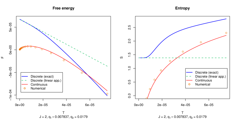
As seen in figure 8, the numerically computed partition function is a good approximation for curves computed assuming continuity, suggesting that the numerical quadrature rule works as if the density of states were continuous, and therefore it is not useful to estimate the ground state of the discrete spectrum, $\Lambda^{*}$ and $S^{*}$.

It is worth emphasizing the different behavior of the thermodynamic magnitudes between the discrete and continuous systems. Any computation method for $Z$ should respect the discrete nature of the spectrum. Otherwise the method would accurately compute the result (92).

Nevertheless, the two behaviors coincide at high temperatures, suggesting that there is a crossing temperature $T^{*}$ below which the difference becomes drastic. Of course, in figure 8 (right) we can see that the entropy of the discrete system (obtained by exact computation of $Z$ using brute-force compilation of states) and the approximate one (that of the continuous system) never cross. But if we approximate the former using the approximated free energy (83), then we can find a temperature at which the continuous and discrete entropies coincide. This temperature $T^{*}$ signals the point of a drastic deviation of the discrete system from the continuous one, and it will be interpreted as an estimator for the ground state $\Lambda^{*}$.

Thus, we need the entropy in (92), which will be termed $S_{\text{cont}}$, and the entropy derived from (83), which is

$$S_{\text{disc}}=S^{*}+\log\Bigl{(}1+e^{\hat{S}-S^{*}}e^{-\frac{\delta\Lambda}{T}}\Bigr{)}+\frac{\delta\Lambda e^{\hat{S}-S^{*}}e^{-\frac{\delta\Lambda}{T}}}{T\bigl{(}1+e^{\hat{S}-S^{*}}e^{-\frac{\delta\Lambda}{T}}\bigr{)}}\,.$$ (93)

The crossing temperature is defined by the equation $S_{\text{disc}}=S_{\text{cont}}$, but (93) contains the degeneracy entropies $S^{*}$, $\hat{S}$ and the gap $\delta\Lambda$ as additional parameters. Of course, we cannot use a single equation to fix four parameters; we will compute the degeneracies as $2^{J\alpha^{*}}$ for the case of incommensurate charges (that is, $S^{*}=\hat{S}$), and we will introduce the parameter $\eta=\frac{\delta\Lambda}{T^{*}}$, so that the equation for $T^{*}$ reads

$$S^{*}+\log\bigl{(}1+e^{-\eta}\bigr{)}+\frac{\eta}{1+e^{\eta}}=1+\log\frac{T^{*}\omega_{J}(R)}{R}$$ (94)

and gets solved as

$$T^{*}=e^{S^{*}}\frac{R}{\omega_{J}(R)}\bigl{(}1+e^{-\eta}\bigr{)}\,e^{\frac{\eta}{1+e^{\eta}}-1}\,.$$ (95)

In terms of the previous estimator $\Lambda_{\varepsilon}$ (79), we have

$$T^{*}(\eta)=f(\eta)\Lambda_{\varepsilon}\,,\quad\text{with}\quad f(\eta)=\bigl{(}1+e^{-\eta}\bigr{)}\,e^{\frac{\eta}{1+e^{\eta}}-1}\,,$$ (96)

where the prefactor $f(\eta)$ is of order $\mathcal{O}(1)$ for $0<\eta<\infty$: it is a monotonically decreasing function with $f(0)=2e^{-1}$ and $f(\infty)=e^{-1}$. Thus, when we let $\eta$ run across its range, the estimator $T^{*}(\eta)$ spans the interval $[1,2]e^{-1}\Lambda_{\varepsilon}$ instead of the single value $\Lambda_{\varepsilon}$. Nevertheless, we cannot give an argument which favours the inclusion of the true value inside this interval. Despite this uncertainty, our numerical searches validate the given interval for $J=2$ and $J=3$: it contains the median and its width is smaller than the interquartile range (see figure 7).

Thus, we can conclude that $T^{*}$ is a good estimator of the charge-averaged minimum cosmological constant.

3.4 A possible influence on the KKLT mechanism

The exposition in this paper is restricted to the Bousso-Polchinski Landscape, which is an oversimplification of the string theory Landscape. The Giddings-Kachru-Polchinski model [26] is a more realistic approach to the true Landscape, and it can be endowed with a mechanism for fixing the moduli of the compactification manifold, the so-called KKLT mechanism [27]. In this model, the compactification moduli are fixed by the presence of fluxes and corrections to the superpotential coming from localized branes. The fixing of the moduli lead to metastable dS states by the addition of anti-branes and exceeding flux. The model can be further corrected to yield inflation of the noncompact geometry by the repulsion between a brane and an antibrane, both located at a Klevanov-Strassler throat [28]. The important point is that both moduli fixing and brane inflation need the presence of flux quanta.

As far as we know, there is no combination between the BP Landscape and the KKLT mechanism, in the sense that there is no known realistic model in which all moduli are fixed and a large amount of three-cycles lead to an anthropic value of the cosmological constant without any fine-tuning at all. Nevertheless, there are some toy models as the six-dimensional Einstein-Maxwell theory [29, 30] in which it is possible to identify a Landscape with all moduli fixed, and it has a dual model with flux; or the more sophisticated (yet unrealistic as well) models coming from F-theory flux compactification [31] or IIB compactifications with fluxes [32], to name a few. Thus, it is plausible that a complete, realistic model exhibiting all these features will be built in the near future.

Let us assume that such a model exists. Furthermore, let us assume that the $\alpha^{*}(h)$ curve discussed in the section 3.2 can be generalized, in the sense that, as a characteristic feature of this conjecturally realistic model of the string theory Landscape, there is a typical occupation number of the fluxes that is generically different from 1 and that vanishes when the number of fluxes $J$ is too large. Then, we should conclude that, generically, there will be a finite fraction $1-\alpha^{*}$ of three-cycles with vanishing flux, which may be dominant if $J$ is large and the charges $q_{i}$ are not too small. This fraction of vanishing fluxes can spoil the stabilization mechanism of the corresponding moduli and can also spoil the brane inflation scenario if the three-cycles located at the tip of the KS throats are devoid of flux.

Thus, the $\alpha^{*}$ fraction we have found in the BP Landscape can be an obstacle for the commonly accepted KKLT mechanism if it is also present in a realistic Landscape model.

4 Conclusions

We have developed an exact formula for counting states in the Bousso-Polchinski Landscape which reduces to the volume-counting one in certain (BP) regime. The formula might be useful in BP Landscape examples when the parameter $h=\frac{Jq^{2}}{r^{2}}$ is large enough to invalidate the BP count. Applications of the formula are given which avoid volume-counting: counting low-lying states, computing the typical fraction of non-vanishing fluxes or estimating the minimum value of the cosmological constant which can be achieved in the BP Landscape. Numeric computations and brute-force searches have been carried out to check the results of our analytic approximations, and we have found remarkable agreement in all explored regimes.

In particular, we have discovered a robust property of the BP Landscape, the curve $\alpha^{*}(h)$, the typical fraction of non-vanishing fluxes, which reveals the structure of the lattice inside a sphere for large $J$ as the union of hyperplane portions of effective dimension near $J\alpha^{*}$. This result is important in computing degeneracies, which are used in estimating the minimum cosmological constant. We have not developed a formula for this minimum, not even a probability distribution, but rather an estimator which can produce acceptable results in predicting the mean value of the minimum for fluctuating different charges around its geometric mean, or essential degeneracies in the case of equal charges.

Finally, we have pointed out that if we can generalize the typical number of non-vanishing fluxes in a realistic model describing the string theory Landscape, then it could be an obstacle for the implementation in the same hypotetical model of the KKTL moduli stabilization mechanism.

Thus, the exact formula improves the way of counting as compared to previous proposals, and should be considered in all those problems which require state enumeration in the BP Landscape.

Appendix A Detailed computation of the typical fraction of non-vanishing fluxes

Consider an arbitrary subset of nodes in the lattice $\Sigma\subset\mathcal{L}$. We will decompose its cardinality $|\Sigma|=\mathcal{N}_{\Sigma}$ as

$$\mathcal{N}_{\Sigma}=\sum_{j=0}^{J}\mathcal{N}_{\Sigma}(j)\,,$$ (97)

where $\mathcal{N}_{\Sigma}(j)$ is the number of states in $\Sigma$ with exactly $j$ non-vanishing components. If $\alpha$ is the fraction $\frac{j}{J}$ then its probability distribution over $\Sigma$ is

$$P_{\Sigma}\bigl{(}\alpha={\textstyle\frac{j}{J}}\bigr{)}=\frac{\mathcal{N}_{\Sigma}(j)}{\mathcal{N}_{\Sigma}}\,.$$ (98)

This formula takes into account only abundances of states in $\Sigma$, and hence it assumes that all states in $\Sigma$ are equally probable.

Let us introduce some notation. We will call the set of indexes of components $\mathcal{J}=\{1,2,\cdots,J\}$ and $L,M$ will denote any subset of $\mathcal{J}$. The symbol $\Sigma_{L}$ will denote the set of states of $\Sigma$ having (at least) vanishing components outside $L$ or, in other words, the intersection between $\Sigma$ and the subspace spanned by the directions in $L$. $\mathcal{N}_{L}$ will be the number of elements of $\Sigma_{L}$. Thus, $\Sigma_{\mathcal{J}}$ comprises all $\Sigma$ states, that is, $\mathcal{N}_{\mathcal{J}}=\mathcal{N}_{\Sigma}$, and $\Sigma_{\emptyset}$ only contains the node at the origin, so that $\mathcal{N}_{\emptyset}=1$. The inclusion-exclusion principle in Combinatorics allows us to write

$$\mathcal{N}_{\Sigma}(j)=\sum_{\begin{subarray}{c}L\subset\mathcal{J}\\ |L|=j\end{subarray}}\sum_{\ell=1}^{j}(-1)^{j-\ell}\sum_{\begin{subarray}{c}M\subset L\\ |M|=\ell\end{subarray}}\mathcal{N}_{M}\,.$$ (99)

The idea behind (99) is that we cannot simply sum all states lying inside every $\Sigma_{L}\in\Sigma$, that is, equation $\mathcal{N}_{\Sigma}(j)=\sum_{\begin{subarray}{c}L\subset\mathcal{J}\\ |L|=j\end{subarray}}\mathcal{N}_{L}$ is not true, because of the intersections between different subsets $\Sigma_{L}$. The nodes inside these intersections are removed twice, and they should be added again, and so on. This is the cause of the alternating sign in (99).

Now, we must deal with expressions of the form

$$\sum_{\begin{subarray}{c}L\subset\mathcal{J}\\ |L|=j\end{subarray}}\sum_{\begin{subarray}{c}M\subset L\\ |M|=\ell\end{subarray}}\mathcal{N}_{M}\,.$$ (100)

All the subsets $M\subset\mathcal{J}$ occur in the previous sum the same number of times, which coincides with the number of supersets $L$ inside $\mathcal{J}$ (with $|L|=j$) of a given $M$ (with $|M|=\ell<j$). This can be computed as the number of subsets of $\mathcal{J}\backslash M$ of exactly $j-\ell$ elements, that is,

$$\sum_{\begin{subarray}{c}L\subset\mathcal{J}\\ |L|=j\end{subarray}}\sum_{\begin{subarray}{c}M\subset L\\ |M|=\ell\end{subarray}}\mathcal{N}_{M}=\binom{J-\ell}{j-\ell}\sum_{\begin{subarray}{c}M\subset\mathcal{J}\\ |M|=\ell\end{subarray}}\mathcal{N}_{M}\,.$$ (101)

By substituting (101) in (99), we get

$$\mathcal{N}_{\Sigma}(j)=\sum^{j}_{\ell=1}(-1)^{j-\ell}\binom{J-\ell}{j-\ell}\sum_{\begin{subarray}{c}M\subset\mathcal{J}\\ |M|=\ell\end{subarray}}\mathcal{N}_{M}\,.$$ (102)

We can check that equation (102) satisfies the normalization condition (97):

$$\begin{split}\sum^{J}_{j=0}\mathcal{N}_{\Sigma}(j)&=\sum^{J}_{j=0}\sum^{j}_{\ell=1}(-1)^{j-\ell}\binom{J-\ell}{j-\ell}\sum_{\begin{subarray}{c}M\subset\mathcal{J}\\ |M|=\ell\end{subarray}}\mathcal{N}_{M}\\ &=\sum^{J}_{\ell=0}\underbrace{\Biggl{[}\sum^{J}_{j=\ell}(-1)^{j-\ell}\binom{J-\ell}{j-\ell}\Biggr{]}}_{\sum^{J-\ell}_{k=0}(-1)^{k}\binom{J-\ell}{k}=\delta_{J,\ell}}\sum_{\begin{subarray}{c}M\subset\mathcal{J}\\ |M|=\ell\end{subarray}}\mathcal{N}_{M}\\ &=\sum_{\begin{subarray}{c}M\subset\mathcal{J}\\ |M|=J\end{subarray}}\mathcal{N}_{M}=\mathcal{N}_{\mathcal{J}}=\mathcal{N}_{\Sigma}\,.\end{split}$$ (103)

Now, we will take the $\Sigma$ set as the states of the lattice $\mathcal{L}$ near the $\Lambda=0$ surface, inside a thin shell of width $\Lambda_{\varepsilon}$, whose number is (100)

$$\mathcal{N}_{\Sigma}=\frac{\omega_{J}(R)}{R}\Lambda_{\varepsilon}\,.$$ (104)

With different charges $q_{i}$, different subsets $M\in\mathcal{J}$ with the same cardinality $|M|=\ell$ will not have the same number of states $\mathcal{N}_{M}$. However, in the simplest case where all charges are equal, all the number of states coincide:

$$\sum_{\begin{subarray}{c}M\subset\mathcal{J}\\ |M|=\ell\end{subarray}}\mathcal{N}_{M}=\binom{J}{\ell}\frac{\omega_{\ell}(R)}{R}\Lambda_{\varepsilon}\,,$$ (105)

where we have used that there is $\binom{J}{\ell}$ different subsets $M\in\mathcal{J}$ with $|M|=\ell$. Substituting (105) in (102) and reordering the binomial coefficients we have

$$\begin{split}\mathcal{N}_{\Sigma}(j)&=\sum^{j}_{\ell=1}(-1)^{j-\ell}\binom{J-\ell}{j-\ell}\binom{J}{\ell}\frac{\omega_{\ell}(R)}{R}\Lambda_{\varepsilon}\\ &=\frac{\Lambda_{\varepsilon}}{R}\binom{J}{j}\sum^{j}_{\ell=1}\binom{j}{\ell}(-1)^{j-\ell}\omega_{\ell}(R)\,.\end{split}$$ (106)

Now, we can substitute the exact integral representation (27) specialized for equal charges for $\omega_{\ell}(R)$ and perform the binomial sum:

$$\begin{split}\mathcal{N}_{\Sigma}(j)&=\frac{\Lambda_{\varepsilon}}{R}\binom{J}{j}\frac{2R}{2\pi i}\int_{\gamma}e^{sR^{2}}\biggl{[}\sum^{j}_{\ell=0}\binom{j}{\ell}(-1)^{j-\ell}\vartheta(q^{2}s)^{\ell}\biggr{]}\,{\rm d}s\\ &=\frac{2\Lambda_{\varepsilon}}{2\pi i}\binom{J}{j}\int_{\gamma}e^{sR^{2}}\bigl{[}\vartheta(q^{2}s)-1\bigr{]}^{j}\,{\rm d}s\,.\end{split}$$ (107)

Normalization provides the probability distribution of $\alpha=\frac{j}{J}$ we are looking for:

$$P(\alpha)=\frac{2R}{\omega_{J}(R)}\binom{J}{\alpha J}\frac{1}{2\pi i}\int_{\gamma}e^{\phi(s,\alpha)}\,{\rm d}s\quad\text{with}\quad\phi(s,\alpha)=sR^{2}+\alpha J\log\bigl{[}\vartheta(q^{2}s)-1\bigr{]}\,.$$ (108)

The next step is estimating $P(\alpha)$ using the steepest descent method again. The equation for the saddle point is

$$\phi^{\prime}(s)=R^{2}+\alpha Jq^{2}\frac{\vartheta^{\prime}(q^{2}s)}{\vartheta(q^{2}s)-1}=0\,.$$ (109)

As we did before, we can find approximate expressions for the saddle point in the two regimes of $\vartheta$ function. If $s^{*}$ is the saddle point, convenient variables are $\upsilon=q^{2}s^{*}$ and $h=\frac{Jq^{2}}{R^{2}}$, in terms of which we have

$$\phi(\upsilon)=\frac{R^{2}}{q^{2}}\Bigl{[}\upsilon+h\alpha\log\bigl{[}\theta(\upsilon)-1\bigr{]}\Bigr{]}\,.$$ (110)

In the large $\upsilon$ regime, we have $\vartheta(\upsilon)\approx 1+2e^{-\upsilon}+2e^{-4\upsilon}$, so that

$$\begin{split}\phi(\upsilon)&\approx\frac{R^{2}}{q^{2}}\Bigl{[}\upsilon+h\alpha\bigl{(}-\upsilon+\log 2+\log(1+e^{-3\upsilon})\bigr{)}\Bigr{]}\\ &\approx\frac{R^{2}}{q^{2}}\Bigl{[}\upsilon(1-h\alpha)+h\alpha\log 2+h\alpha e^{-3\upsilon}\Bigr{]}\,,\end{split}$$ (111)

and the corresponding saddle point equation has a solution

$$\upsilon(h\alpha)=-\frac{1}{3}\log\frac{1}{3}\Bigl{(}\frac{1}{h\alpha}-1\Bigr{)}\,.$$ (112)

In the small $\upsilon$ regime, we simply have $\vartheta(\upsilon)\approx\sqrt{\frac{\pi}{\upsilon}}$, so that

$$\begin{split}\phi(\upsilon)&\approx\frac{R^{2}}{q^{2}}\Bigl{[}\upsilon+h\alpha\Bigl{[}\textstyle\frac{1}{2}\log\pi-\frac{1}{2}\log\upsilon+\log\Bigl{(}1-\sqrt{\frac{\upsilon}{\pi}}\Bigr{)}\Bigr{]}\Bigr{]}\\ &\approx\frac{R^{2}}{q^{2}}\Bigl{[}\upsilon+h\alpha\Bigl{[}\textstyle{\frac{1}{2}\log\pi-\frac{1}{2}\log\upsilon}-\sqrt{\frac{\upsilon}{\pi}}-\frac{\upsilon}{2\pi}\Bigr{]}\Bigr{]}\,.\end{split}$$ (113)

The corresponding saddle point equation is quadratic in $\frac{1}{\sqrt{\upsilon}}$, and its solution is

$$\upsilon(h\alpha)\approx\frac{4\pi}{\Bigl{(}\sqrt{\frac{8\pi}{h\alpha}-3}-1\Bigr{)}^{2}}\approx\frac{h\alpha}{2}+\sqrt{\frac{2}{\pi}}\frac{(h\alpha)^{\frac{3}{2}}}{4}+\frac{3(h\alpha)^{2}}{8\pi}+\cdots$$ (114)

Both approximate solutions (112) and (114), as well as a numerical one, are plotted in figure 9.

Figure 9: Numerical saddle point $\upsilon(h\alpha)$ of the $P(\alpha)$ integrand for equal charges along with its two asymptotic regimes.

Note the logarithmic divergence at $h\alpha=1$ of the saddle point. For larger values, $\upsilon(h\alpha)$ becomes complex, and the integral $P(\alpha)$ begins to oscillate, losing its probabilistic meaning.

Using the asymptotic form of the binomial coefficient, we can write

$$P(\alpha)\propto e^{Js(\alpha)}\quad\text{with}\quad s(\alpha)=-\alpha\log\alpha-(1-\alpha)\log(1-\alpha)+\frac{1}{J}\phi(\upsilon,\alpha)\,,$$ (115)

where $\phi(\upsilon,\alpha)$ also depends implicitly on $\alpha$ through $\upsilon$. The exponent $s(\alpha)$ has a maximum $\alpha^{*}$, given by the equation

$$\begin{split}\frac{\,{\rm d}s}{\,{\rm d}\alpha}&=-\log\alpha+\log(1-\alpha)+\underbrace{\frac{\partial\phi}{\partial\upsilon}}_{=0}\frac{\,{\rm d}\upsilon}{\,{\rm d}\alpha}+\frac{\partial\phi}{\partial\alpha}\\ &=\log\frac{1-\alpha}{\alpha}+\log\bigl{[}\vartheta\bigl{(}\upsilon(h\alpha)\bigr{)}-1\bigr{]}=0\,.\end{split}$$ (116)

In the first equality of (116) we have used the definition of the saddle point $\upsilon$, and in the second we have used equation (110). We obtain $\alpha^{*}$ as the unique real solution in the $[0,1]$ interval of

$$\vartheta\bigl{[}\upsilon(h\alpha)\bigr{]}=\frac{1}{1-\alpha}\,.$$ (117)

Note that the saddle point $\upsilon(h\alpha)$ is defined only for $h\alpha\leq 1$ (see fig. 9), so that the right hand side of equation (117) as a function of $\alpha$ has domain $\alpha\in[0,\frac{1}{h}]$. In this interval, $\vartheta[\upsilon(h\alpha)]$ decreases from $\infty$ to 1, while the right hand side increases from 1 to $\infty$ in $\alpha\in[0,1]$. These conditions guarantee the existence of a unique real solution $\alpha^{*}(h)\in[0,1]$ for all positive $h$. Figure 10 shows the construction of $\alpha^{*}(h)$.

Figure 10: Construction of the solution $\alpha^{*}$ of equation (117) for $0<h<3$. Dashed curve corresponds to $h=1$. For $h\ll 1$, the solution is near $\alpha=1$, and for $h\gg 1$ the solution approaches zero.

For small $h$, we can use the small $h\alpha$ regime for $\upsilon(h\alpha)$ (eq. (114)) and $\vartheta$ (eq. (32)), in which equation (117) reads

$$\sqrt{\frac{2\pi}{h\alpha}}=\frac{1}{1-\alpha}\,,$$ (118)

and has the solution

$$\alpha^{*}(h)\approx 1-\frac{1}{4\pi}\bigl{[}\sqrt{h(h+8\pi)}-h\bigr{]}\,.$$ (119)

For $h\alpha$ approaching 1, we can use (112) for $\upsilon(h\alpha)$ and the corresponding regime for $\vartheta$, so that (117) simplifies to

$$1+2e^{\frac{1}{3}\log\frac{1}{3}\bigl{(}\frac{1}{h\alpha}-1\bigl{)}}=\frac{1}{1-\alpha}\,.$$ (120)

We can isolate $h(\alpha^{*})$ in (120), obtaining

$$h(\alpha^{*})\approx\frac{1}{\alpha^{*}\bigl{(}1+\frac{3}{8}\,\bigl{(}\frac{\alpha^{*}}{1-\alpha^{*}}\bigr{)}^{3}\bigr{)}}\,,$$ (121)

which for large $h$ is simply $\alpha^{*}\approx\frac{1}{h}$. All these regimes are shown in figure 4 along with the numerical solution of equation (117).

Appendix B Typical fraction of non-vanishing fluxes in the pure BP regime

We can repeat the computation of the probability distribution of the fraction of non-vanishing fluxes $P(\alpha)$ (given in appendix A) in the pure BP regime step by step. Using the previous notation, we will consider all states inside a sphere of radius $r$ as the set $\Sigma\subset\mathcal{L}$, but we will use the BP formula (7) instead of the exact integral representation of the number of such states (hence the name “pure BP”):

$$\mathcal{N}_{\Sigma}=\Omega_{J}(r)\approx\frac{2\pi^{\frac{J}{2}}r^{J}}{J\Gamma\bigl{(}\frac{J}{2}\bigr{)}\operatorname{vol}Q}\,.$$ (122)

The computation of the probability distribution is based in the decomposition (97), which we repeat here for convenience:

$$\mathcal{N}_{\Sigma}=\sum_{j=0}^{J}\mathcal{N}_{\Sigma}(j)\,,$$ (123)

After using the inclusion-exclusion principle, we have (102)

$$\mathcal{N}_{\Sigma}(j)=\sum^{j}_{\ell=1}(-1)^{j-\ell}\binom{J-\ell}{j-\ell}\sum_{\begin{subarray}{c}M\subset\mathcal{J}\\ |M|=\ell\end{subarray}}\mathcal{N}_{M}\,.$$ (124)

As before, we will assume that all charges are equal $\operatorname{vol}Q=q^{J}$. Thus we have an equation analogous to (105)

$$\sum_{\begin{subarray}{c}M\subset\mathcal{J}\\ |M|=\ell\end{subarray}}\mathcal{N}_{M}=\binom{J}{\ell}\frac{\pi^{\frac{\ell}{2}}r^{\ell}}{\Gamma\bigl{(}\frac{\ell}{2}+1\bigr{)}q^{\ell}}=\binom{J}{\ell}\frac{\xi^{\ell}}{\Gamma\bigl{(}\frac{\ell}{2}+1\bigr{)}}\,,$$ (125)

where we have used the parameter

$$\xi=\frac{r\sqrt{\pi}}{q}\,.$$ (126)

Plugging (125) in the decomposition (124),

$$\mathcal{N}_{\Sigma}(j)=\sum^{j}_{\ell=1}(-1)^{j-\ell}\binom{J-\ell}{j-\ell}\binom{J}{\ell}\frac{\xi^{\ell}}{\Gamma\bigl{(}\frac{\ell}{2}+1\bigr{)}}=\binom{J}{j}\sum^{j}_{\ell=1}(-1)^{j-\ell}\binom{j}{\ell}\frac{\xi^{\ell}}{\Gamma\bigl{(}\frac{\ell}{2}+1\bigr{)}}\,.$$ (127)

Now we take the Hankel definition of the gamma function:

$$\frac{1}{\Gamma(x)}=\frac{1}{2\pi i}\int_{C}e^{z}z^{-x}\,{\rm d}z\,,$$ (128)

where the contour $C$ in complex $z$ plane encloses the origin coming from $-\infty$ below the negative real axis, turning around the origin and leaving towards $-\infty$ over the negative real axis. By substituting

$$\frac{1}{\Gamma\bigl{(}\frac{\ell}{2}+1\bigr{)}}=\frac{1}{2\pi i}\int_{C}e^{z}z^{-(\frac{\ell}{2}+1)}\,{\rm d}z$$ (129)

in (127), we can interchange the sum and the integral and the binomial theorem allows us to write

$$\begin{split}\mathcal{N}_{\Sigma}(j)&=\binom{J}{j}\sum^{j}_{\ell=1}(-1)^{j-\ell}\binom{j}{\ell}\xi^{\ell}\frac{1}{2\pi i}\int_{C}e^{z}z^{-(\frac{\ell}{2}+1)}\,{\rm d}z\\ &=\binom{J}{j}\frac{1}{2\pi i}\int_{C}e^{z}\frac{\,{\rm d}z}{z}\sum^{j}_{\ell=1}(-1)^{j-\ell}\binom{j}{\ell}\Bigl{(}\frac{\xi}{\sqrt{z}}\Bigr{)}^{\ell}\\ &=\binom{J}{j}\frac{1}{2\pi i}\int_{C}e^{z}\biggl{(}\frac{\xi}{\sqrt{z}}-1\biggr{)}^{j}\frac{\,{\rm d}z}{z}\,.\end{split}$$ (130)

By changing the $z$ variable to $s=z/\xi^{2}$ the contour only gets scaled and can be deformed back to its original form, resulting in

$$\mathcal{N}_{\Sigma}(j)=\binom{J}{j}\frac{1}{2\pi i}\int_{C}e^{\xi^{2}s}\biggl{(}\frac{1}{\sqrt{s}}-1\biggr{)}^{j}\frac{\,{\rm d}s}{s}=\binom{J}{j}\frac{1}{2\pi i}\int_{C}e^{J\phi(s)}\frac{\,{\rm d}s}{s}\,.$$ (131)

We have defined the function

$$\phi(s)=\frac{\pi s}{h}+\alpha\log\biggl{(}\frac{1}{\sqrt{s}}-1\biggr{)}\,,$$ (132)

which depends on the two parameters mainly used in the remainder of the paper:

$$h=\frac{Jq^{2}}{r^{2}}\qquad\text{and}\qquad\alpha=\frac{j}{J}\,.$$ (133)

Note that $\xi=\sqrt{\frac{J\pi}{h}}$.

We can normalize $\mathcal{N}_{\Sigma}(j)$ dividing by $\mathcal{N}_{\Sigma}$ in (122), thus obtaining the following integral representation for the probability distribution:

$$P(\alpha)=\Gamma\bigl{(}{\textstyle\frac{J}{2}}+1\bigr{)}\xi^{-J}\binom{J}{j}\frac{1}{2\pi i}\int_{C}e^{J\phi(s)}\frac{\,{\rm d}s}{s}\,.$$ (134)

We can evaluate the integral using the steepest descent method, assuming that $J$ is large and that $h$ and $\alpha$ are constant parameters. Furthermore, $h$ cannot be too large for the saddle point approximation to remain valid.

Thus, for large $J$, $P(\alpha)$ is

$$P(\alpha)\propto e^{Js(\alpha)}\qquad\text{with}\qquad s(\alpha)=-\alpha\log\alpha-(1-\alpha)\log(1-\alpha)+\phi(s^{*})\,,$$ (135)

where we have used the asymptotic expression for large $J$ of $\binom{J}{J\alpha}$ and $s^{*}$ is the saddle point of $\phi(s)$ which is compatible with the integration contour $C$. We compute $s^{*}$ as a solution of

$$\phi^{\prime}(s)=\frac{\pi}{h}-\frac{\alpha}{2}\,\frac{1}{s(1-\sqrt{s})}=0\,,$$ (136)

which can be rewritten as

$$s\sqrt{s}-s+\nu=0\,,$$ (137)

with the new parameter $\nu=\frac{h\alpha}{2\pi}$. Let us assume for simplicity that $\nu$ is small (that is, $h$ is small); then (137) has two solutions in the positive real axis, one of them near 0 and the other near 1. Near $s\approx 0$, $\phi^{\prime\prime}(s)\approx\frac{\alpha}{2s^{2}}>0$ and near $s\approx 1$, $\phi^{\prime\prime}(s)\approx\frac{-\alpha}{4\sqrt{s}(1-\sqrt{s})^{2}}<0$, so the first corresponds to a local minimum over the positive real axis and the second to a local maximum. But the integration contour crosses the positive real axis vertically from lower to upper half plane, and therefore the integrand has a maximum along $C$ if it has a minimum along the real axis. So our saddle point is near 0 for small $\nu$, and it follows from (137) that we must have

$$s^{*}\xrightarrow{\nu\to 0}\nu\,.$$ (138)

We can find the maximum of the “entropy” $s(\alpha)$ in (135), which we will call $\alpha^{*}$, by solving the stationary condition

$$\frac{\,{\rm d}s(\alpha)}{\,{\rm d}\alpha}=\log\frac{1-\alpha}{\alpha}+\underbrace{\frac{\partial\phi(s)}{\partial s}\Bigl{|}_{s=s^{*}}}_{0}\frac{\,{\rm d}s^{*}}{\,{\rm d}\alpha}+\frac{\partial\phi(s)}{\partial\alpha}\Bigl{|}_{s=s^{*}}=\log\frac{1-\alpha}{\alpha}+\log\biggl{(}\frac{1}{\sqrt{s^{*}}}-1\biggr{)}=0\,.$$ (139)

With the estimate (138) for small $\nu$, eq. (139) can be rewritten as

$$\frac{1-\alpha}{\alpha}\approx\sqrt{\nu}\,.$$ (140)

In the preceding equation, if $\nu$ is small, then its solution $\alpha^{*}$ must be near 1; replacing $\alpha\approx 1$ in the denominator of (140) we obtain exactly (118), which determines $\alpha^{*}(h)$ for small $h$. So this approach ends up with the same estimate for the typical fraction of non-vanishing fluxes for small $h$, despite the fact that we are computing this fraction $\alpha^{*}$ over the whole Landscape instead of over a thin shell. This is a strong indication that the result obtained for $\alpha^{*}$ is robust, in the sense that it does not change significantly for different generic subsets of the Landscape.

We remark that the robustness of the $\alpha^{*}(h)$ curve is not a feature of spherical symmetry. This is exemplified by the set of secant states, which is not spherically symmetric [23, 24]. If we repeat the computation in this appendix taking the set of secant states at distance $r$ as the subset $\Sigma\subset\mathcal{L}$ instead of the ball of radius $r$, we would obtain the same estimate. Thus, we should consider $\alpha^{*}(h)$ a robust property of the BP Landscape.

The preceding computation used the BP regime (122), and we have mentioned above that $h$ should be small for the validity of the saddle-point approximation. Now we can wonder, how big can $h$ be before invalidating the approximation. Can we somehow continue this result to higher values of $h$?

The answer to this latter question is negative, as can be seen in figure 11, which, in turn, answers also the former question.

Figure 11: Evolution in complex $s$-plane of the critical points of the $\phi$ function (132), exponent of the integral representation of $P(\alpha)$ in the pure BP regime, versus the $\nu$ parameter. The saddle point $s^{*}$ plotted in red (which begins at $s=0$ and enters the lower half plane for $\nu>\frac{4}{27}$) is compatible with the integration contour $C$, which means that $C$ can be deformed to coincide with the steepest descent contour crossing trough $s^{*}$.

In figure 11 we show the saddle points of $\phi(s)$ as they evolve in complex $s$-plane from $\nu=0$ to $\nu=4$. Both of them start at $s=0,1$ respectively for $\nu=0$ and evolve along the positive real axis until they coincide at $s=\frac{4}{9}$ for $\nu=\frac{4}{27}$. This coincidence can be seen by writing (137) in a variable $x=\sqrt{s}$ and considering its derivative, which is a polynomial whose roots $x^{*}$ are the critical points of $p(x)$:

$$p(x)=x^{3}-x^{2}+\nu\xrightarrow{\frac{\,{\rm d}}{\,{\rm d}x}}3x^{2}-2x=0\quad\Rightarrow\quad x^{*}\in\Bigl{\{}0,\frac{2}{3}\Bigr{\}}\quad\Rightarrow\quad p(x^{*})\in\Bigl{\{}\nu,\nu-\frac{4}{27}\Bigr{\}}\,,$$ (141)

that is, $p(x)$ has two critical points with values above and below the $x$-axis only if $\nu<\frac{4}{27}$. For $\nu>\frac{4}{27}$ both critical points have positive values, and the roots of $p(x)$ leave the real axis.

Only the root near 0 is compatible with the integration contour $C$, that is, $C$ can be deformed to meet the steepest descent contour crossing by the saddle point near $s=0$. For $\nu>\frac{4}{27}$ both roots leave the real axis; as a consequence, the integral $P(\alpha)$ remains real but becomes non-positive and rapidly oscillating, thereby losing its meaning as a probability distribution. Therefore, the pure BP regime is only valid for $\nu<\frac{4}{27}$, that is, for

$$h<\frac{8\pi}{27}=0.93084\,.$$ (142)

This value represents the upper limit of validity of the pure BP regime in the computation of $P(\alpha)$. We can intuitively understand the existence of this limit by considering that the inclusion-exclusion principle (124), being an alternating sum, is very sensitive to inaccurate computations of the cardinals of the subsets appearing in the sum. Therefore, when we use the BP formula (122) for computing the cardinals of the subsets with growing $h$, that is, for decreasing $r$, the error in the formula causes strong oscillations in $P(\alpha)$.

References

- [1] A. H. Guth: The Inflationary Universe: A Possible Solution to the Horizon and Flatness Problems. Phys. Rev. D 23: 347-356 (1981).
- [2] A. D. Linde: A New Inflationary Universe Scenario: A Possible Solution of the Horizon, Flatness, Homogeneity, Isotropy and Primordial Monopole Problems. Phys. Lett. B 108: 389-393 (1982).
- [3] A. D. Linde: Chaotic Inflation. Phys. Lett. B 129: 177-181 (1983).
- [4] A. D. Linde: Eternal Chaotic Inflation. Mod. Phys. Lett. A 1: 81 (1986).
- [5] A. H. Guth: Inflation and Eternal Inflation. Phys. Rept. 333: 555-574 (2000). arXiv:astro-ph/0002156
- [6] J. D. Brown and C. Teitelboim: Dynamical neutralization of the cosmological constant. Phys. Lett. B195, 177 (1987).
- [7] J. D. Brown and C. Teitelboim: Neutralization of the cosmological constant by membrane creation. Nucl. Phys. B297, 787-836 (1988).
- [8] Supernova Cosmology Project (S. Perlmutter et al.): Measurements of and from 42 high redshift supernovae. Astrophys. J. 517: 565-586 (1999). arXiv:astro-ph/9812133
- [9] Supernova Search Team (Adam G. Riess et al.): Observational evidence from supernovae for an accelerating universe and a cosmological constant. Astron. J. 116: 1009-1038 (1998). arXiv:astro-ph/9805201
- [10] J. D. Barrow and F. J. Tipler: The Anthropic Cosmological Principle. Oxford University Press (1986), sec. 6.9, 6.10.
- [11] S. Weinberg: Anthropic Bound on the Cosmological Constant. Phys. Rev. Lett. 59, 2607-2610 (1987).
- [12] L. Susskind: The Anthropic Landscape of String Theory. arXiv:hep-th/0302219
- [13] S. Weinberg: The cosmological constant problem. Rev. Mod. Phys. 61, 1-23 (1989).
- [14] R. Bousso: TASI Lectures on the Cosmological Constant. Gen. Rel. Grav. 40: 607 (2008). arXiv:0708.4231 [hep-th]
- [15] R. Bousso and J. Polchinski: Quantization of four-form fluxes and dynamical neutralization of the cosmological constant. JHEP 06: 006 (2000). arXiv:hep-th/0004134
- [16] T. Clifton, S. Shenker and N. Sivanandam: Volume Weighted Measures of Eternal Inflation in the Bousso-Polchinski Landscape. JHEP 0709: 034 (2007). arXiv:0706.3201 [hep-th]
- [17] R. Bousso and I. Yang: Landscape predictions from cosmological vacuum selection. Phys. Rev. D 75: 123520 (2007). arXiv:hep-th/0703206
- [18] S. Ashok and M. R. Douglas: Counting flux vacua. JHEP 0401: 060 (2004). arXiv:hep-th/0307049
- [19] M. R. Douglas: Basic results in vacuum statistics. Comptes Rendus Physique 5: 965-977 (2004). arXiv:hep-th/0409207
- [20] M. R. Douglas: The Statistics of string / M theory vacua. JHEP 0305: 046 (2003). arXiv:hep-th/0303194
- [21] R. Bousso: Precision cosmology and the landscape. arXiv:hep-th/0610211
- [22] D. Schwartz-Perlov and A. Vilenkin: Probabilities in the Bousso-Polchinski multiverse. JCAP 0606: 010 (2006). arXiv:hep-th/0601162
- [23] C. Asensio and A. Segui: A geometric-probabilistic method for counting low-lying states in the Bousso-Polchinski Landscape. Phys. Rev. D 80: 043515 (2009). arXiv:0812.3247 [hep-th]
- [24] C. Asensio and A. Segui: Counting states in the Bousso-Polchinski Landscape, 99-110 in M. Asorey, J. V. García Esteve, M. F. Rañada and J. Sesma (Editors): Mathematical Physics and Field Theory – Julio Abad, in Memoriam, Prensas Universitarias de Zaragoza, ISBN 978-84-92774-04-3 (2009). arXiv:0903.1947 [hep-th]
- [25] R Development Core Team: R: A language and environment for statistical computing. R Foundation for Statistical Computing, Vienna, Austria. ISBN 3-900051-07-0 (2007). http://www.R-project.org
- [26] S. B. Giddings, S. Kachru and J. Polchinski: Hierarchies from fluxes in string compactifications. Phys. Rev. D 66: 106006 (2002). arXiv:hep-th/0105097
- [27] S. Kachru, R. Kallosh, A. Linde and S. Trivedi: de Sitter vacua in string theory. Phys. Rev. D 68: 046005 (2003). arXiv:hep-th/0301240
- [28] S. Kachru, R. Kallosh, A. Linde, J. Maldacena, L. McAllister and S. Trivedi: Towards inflation in string theory. JCAP 0310: 013 (2006). arXiv:hep-th/0308055
- [29] M. R. Douglas and S. Kachru: Flux compactifications. Rev. Mod. Phys. 79: 733-796 (2007). arXiv:hep-th/0610102
- [30] J. J. Blanco-Pillado, D. Schwartz-Perlov and A. Vilenkin: Quantum tunneling in flux compactifications. JCAP 0912: 006 (2009). arXiv:0904.3106 [hep-th]
- [31] F. Denef, M. R. Douglas, B. Florea, A. Grassi and S. Kachru: Fixing all moduli in a simple F-theory compactification. Adv. Theor. Math. Phys. 9: 861-929 (2005). arXiv:hep-th/0503124
- [32] S. Kachru, M. B. Schulz and S. Trivedi: Moduli stabilization from fluxes in a simple IIB orientifold. JHEP 0310: 007 (2003). arXiv:hep-th/0201028